|
CGAL 6.1 - 2D Arrangements
|
|
CGAL 6.1 - 2D Arrangements
|
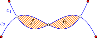
Geometric arrangements, or arrangements for short, are subdivisions of some space induced by geometric objects. Figure 35.1 shows an arrangement of two curves \(c_1\) and \(c_2\) in the plane. It has three faces—two bounded faces \(f_1\) and \(f_2\) (filled with diagonal-stripe patterns) and an unbounded face. The arrangement has seven vertices—four represent the endpoints of \(c_1\) and \(c_2\) (drawn as small discs), and three represent the intersection points of the two curves (drawn as small rings). The arrangement also has eight edges, each of which is a maximal portion of one curve not intersecting the other.
Arrangements are not restricted to curves in the plane. There are useful arrangements in three and higher dimensions (these are not so easy to visualize) and they can be induced by geometric objects of any type, such as spheres, simplices, polytopes, or Bézier surfaces. This package provides a data structure that represents a two-dimensional arrangement of curves embedded in an orientable parametric surface in three dimensional space, such as a plane, a cylinder, a sphere, a torus, or a surface homeomorphic to them. This package also provides operations that construct and manipulate such arrangements. Arrangements are ubiquitous in the computational-geometry literature and have many applications; see, e.g., [1], [3], [4], and [8].
The use of the generic programming paradigm enables a convenient separation of the topology and the geometry of data structures.In this context, we sometimes say combinatorics instead of topology, and say algebra or numerics instead of geometry. We always mean the same thing—the separation of the abstract, graph-like structure (the topology) from the actual embedding in the plane (the geometry). This is a key aspect in the design of geometric software, and is put into practice, for example, in the design of CGAL polyhedra, CGAL triangulations, and our CGAL arrangements. This separation allows the convenient abstraction of algorithms and data structures in combinatorial and topological terms, regardless of the specific geometry of the objects at hand. This abstraction is realized through class and function templates that represent specific data structures and algorithmic frameworks, respectively. Consider the class template
An instance of this template represents an arrangement embedded in the plane. When the template is instantiated, the GeometryTraits parameter must be substituted by a type that defines a set of geometric-object types, such as point and curve, and a set of operations on objects of these types (see Section The Geometry Traits); the Dcel parameter must be substituted by a type that represents a doubly-connected edge list (DCEL) data structure. It defines types of topological objects, such as vertices, edges, and faces, and the operations required to maintain the incidence relations among objects of these types (see Section Representation of Arrangements: The Dcel).
The class template Arrangement_2 derives from the following class template:
An instance of this template represents a two-dimensional arrangement embedded in a surface in three dimensional space. When the template is instantiated, the GeometryTraits parameter must be substituted as described above; the TopologyTraits parameter must be substituted by a type that deals with the topology of the surface (see Section The Topology Traits). In particular, it maintains a representation of the arrangement graph embedded in the surface using a doubly-connected edge list (DCEL) data-structure suitable for the particular topology.
Several member functions and nested types defined in the Arrangement_2 derived class-template inherit their definitions from the base class-template Arrangement_on_surface_2; their semantics is equivalent in both class templates. The names of these member functions and nested types typically appear in the manual without any scope, as each of these class templates can serve as their scope. (As a matter of fact, the package provides additional class templates that represent two-dimensional arrangements, such as the Arrangement_with_history_2 class template, which derives from the class template Arrangement_2; these additional class templates also contain inherited definitions of the aforementioned member functions and nested types.)
An immediate advantage of the separation of the topology and the geometry of data structures is that users with limited expertise in computational geometry can employ the data structure with their own special type of objects. They must, however, supply the relevant traits class, which mainly involves algebraic computations. A traits class also encapsulates the number types used to represent coordinates of geometric objects and to carry out algebraic operations on them. It encapsulates the type of coordinate system used (e.g., Cartesian and homogeneous), and the geometric or algebraic computation methods themselves. The precise minimal sets of requirements the actual traits classes must conform to are organized as a hierarchy of concepts; see Section The Geometry Traits.
What constitutes valid curves that can be handled by the 2D Arrangements package is discussed in detail in Section The Geometry Traits, where the models of the traits classes are described. However, when we cite combinatorial complexity bounds or bounds on the resources (i.e., running time and storage space) required by algorithms, we often postulate stricter assumptions on the input curves. The prevalent term in use is that the curves are well behaved, which may have different interpretations in different settings. If we are concerned with combinatorial complexity bounds for curves embedded in a two-dimensional surface, then the standard assumptions are that (i) each curve is non-self-intersecting (a so-called Jordan arc) and (ii) every pair of curves intersects in at most some constant number of points. For algorithmic purposes we need to require more since we assume that any operation on a small constant number of curves takes unit time. In this sense arcs of algebraic curves of degree bounded by a constant (namely the zero set of bivariate polynomials of constant maximum total degree) are well behaved. Naturally, what are typically considered well-behaved surfaces in \(\mathbb{R}^3\) is even more complicated to state.
Remarks
From the complexity-bound perspective, most of the arrangements that we can deal with can be regarded as defined by well-behaved curves. Even though the package allows for self-intersecting curves, for most types each curve can be decomposed into a constant number of well-behaved curves, thus having no effect on the asymptotic bounds that we state.
One type of curves that we deal with is special in this sense: polylines, namely concatenations of an unlimited number of line segments; see Section The Polyline Traits Class. A polyline is not well behaved, as it cannot be decomposed into a constant number of constant-descriptive complexity subcurves. Informative bounds for arrangements of polylines are expressed by other parameters in addition to the number of polylines, for example, the total number of segments in all the polylines together. The same holds for the more general type polycurve, which are piecewise curves that are not necessarily linear; see Section The Polycurve Traits Class.
In Section Basic Arrangements we provide the minimum material you need to know in order to use CGAL 2D arrangements in the plane. In Section Arrangements on Curved Surfaces we provide additional material you need to know in order use CGAL 2D arrangements embedded in curved surfaces. Most of the succeeding material is oblivious to the type of the embedding surface. In Section Issuing Queries on an Arrangement we show how queries on an arrangement can be issued. In Section Free Functions we review some useful free (global) functions that operate on arrangements, the most important ones being the free insertion-functions. In Section Arrangements of Unbounded Curves we explain how to construct and manipulate arrangements of unbounded curves. Section The Geometry Traits contains detailed descriptions of the geometric traits concept hierarchy and the various geometric traits classes included in the 2D Arrangements package. The different traits classes enables the construction and manipulation of arrangements of different families of curves. Naturally, here, the embedding surface plays a significant role. In Section The Notification Mechanism we review the notification mechanism that allows external classes to keep track of the changes that an arrangement instance goes through. Section Extending the DCEL explains how to extend the DCEL records, to store extra data with them, and to efficiently update this data. In Section Overlaying Arrangements we introduce the fundamental operation of overlaying two arrangements. Section Storing the Curve History describes a class-template that extends the arrangement by storing additional history records with its curves. In Section Input/Output Streams and Visualization we review the arrangement input/output functions. In Section Adapting to Boost Graphs we describes how to apply the graph algorithms implemented in the Boost Graph Library to arrangement types. Finally, in Section How To Speed Up Your Computation we provide some tips that can be applied to expedite computation.
We start with a formal definition of two-dimensional arrangements, and proceed with an introduction to the data structure used to represent the incidence relations among features of two-dimensional arrangements, namely, the doubly-connected edge list, or DCEL for short. In Section The Arrangement Class Template we describe a central component in the 2D Arrangements package, namely, the Arrangement_2 class-template, which can be used to represent arrangements in the plane.
Given a set \(\mathcal{C}\) of curves embedded in a two-dimensional surface, the arrangement \(\mathcal{A}(\mathcal{C})\) is the subdivision of the surface into zero-dimensional, one-dimensional and two-dimensional cells,We use the term cell to describe the various dimensional entities in the induced subdivision. Sometimes, the term face is used for this purpose in the literature. However, we use the term face to describe a two-dimensional cell. called vertices, edges and faces, respectively, induced by the curves in \(\mathcal{C}\).
In our implementation we use a definition that slightly deviates from the standard definition above for practical reasons. The curves in \(\mathcal{C}\) can intersect each other (a single curve may also be self-intersecting or may comprise several disconnected branches) and are not necessarily \(x\)-monotone.A continuous planar curve \(c\) is \(x\)-monotone if every vertical line intersects it at most once. For example, a non-vertical line segment is always \(x\)-monotone and so is the graph of any continuous function \(y = f(x)\). For convenience, we treat vertical line segments as weakly \(x\)-monotone, as there exists a single vertical line that overlaps them. A circle of radius \(r\) centered at \((x_0, y_0)\) is not \(x\)-monotone, as the vertical line \(x = x_0\) intersects it at \((x_0, y_0 - r)\) and at \((x_0, y_0 + r)\). We construct a collection \(\mathcal{C}''\) of \(x\)-monotone subcurves that are pairwise disjoint in their interiors in two steps as follows. First, we decompose each curve in \(\mathcal{C}\) into maximal \(x\)-monotone subcurves and possibly isolated points, obtaining the collection \(\mathcal{C}'\). Note that an \(x\)-monotone curve cannot be self-intersecting. Then, we decompose each curve in \(\mathcal{C}'\) into maximal connected subcurves not intersecting any other curve (or point) in \(\mathcal{C}'\) in its interior. The collection \(\mathcal{C}''\) contains isolated points, if the collection \(\mathcal{C}'\) contains such points. The arrangement induced by the collection \(\mathcal{C}''\) can be conveniently embedded as a planar graph, the vertices of which are associated with curve endpoints or with isolated points, and the edges of which are associated with subcurves. It is easy to see that the faces of \(\mathcal{A}(\mathcal{C})\) are the same as the faces of \(\mathcal{A}(\mathcal{C}'')\). There are possibly more vertices in \(\mathcal{A}(\mathcal{C}'')\) than in \(\mathcal{A}(\mathcal{C})\)—the vertices where curves were cut into \(x\)-monotone (non-intersecting) pieces; accordingly there may also be more edges in \(\mathcal{A}(\mathcal{C}'')\). This graph can be represented using a doubly-connected edge list data-structure (DCEL), which consists of containers of vertices, edges and faces and maintains the incidence relations among these cells. It is one of a family of combinatorial data structures called halfedge data structures (Hds), which are edge-centered data structures capable of maintaining incidence relations among cells of, for example, planar subdivisions, polyhedra, or other orientable, two-dimensional surfaces embedded in a space of arbitrary dimension. Geometric interpretation is added by classes built on top of the halfedge data structure.
The \(x\)-monotone curves of an arrangement are embedded in a rectangular two-dimensional area called the parameter space. The parameter space is defined as \( X \times Y\), where \( X\) and \( Y\) are open, half-open, or closed intervals with endpoints in the compactified real line \( \mathbb{R} \cup \{-\infty,+\infty\}\). Let \(x_{\rm min}\), \(x_{\rm max}\), \(y_{\rm min}\), and \(y_{\rm max}\) denote the endpoints of \( X\) and \( Y\), respectively. We typically refer to these values as the left, right, bottom, and top sides of the boundary of the parameter space. If the parameter space is, for example, the entire compactified plane, as in the case of arrangements in the plane, \(x_{\rm min} = y_{\rm min} = -\infty\) and \(x_{\rm max} = y_{\rm max} = +\infty\); see Section Arrangements on Curved Surfaces for more details.
The DCEL data-structure represents each edge using a pair of directed halfedges, one going from the \(xy\)-lexicographically smaller (left) endpoint of the curve towards the \(xy\)-lexicographically larger (right) endpoint, and the other, known as its twin halfedge, going in the opposite direction. As each halfedge is directed, it has a source vertex and a target vertex. Halfedges are used to separate faces, and to connect vertices, with the exception of isolated vertices (representing isolated points), which are disconnected. If a vertex \(v\) is the target of a halfedge \(e\), we say that \(v\) and \(e\) are incident to each other. The halfedges incident to a vertex \(v\) form a circular list sorted in a clockwise order around this vertex. (An isolated vertex has no incident halfedges.)
An edge of an arrangement is a maximal portion of a curve between two vertices of the arrangement. Each edge is represented in the DCEL by a pair of twin halfedges. Each halfedge \(e\) stores a pointer to its incident face, which is the face lying to its left. Moreover, every halfedge is followed by another halfedge sharing the same incident face, such that the target vertex of the halfedge is the same as the source vertex of the next halfedge. The halfedges around faces form circular chains, such that all halfedges of a chain are incident to the same face and wind along its boundary. We call such a chain a connected component of the boundary, or CCB for short.
The unique CCB of halfedges winding in a counterclockwise orientation along a face boundary is referred to as the outer CCB of the face. For the time being let us consider only (i) arrangements of bounded curves, such that exactly one unbounded face exists in every arrangement, and (ii) arrangements embedded in the plane, such that every face has at most one outer CCB. The unbounded face does not have an outer boundary. Any other connected component of the boundary of the face is called a hole, or inner CCB, and can be represented as a circular chain of halfedges winding in a clockwise orientation around it. Note that a hole does not necessarily correspond to a face at all, as it may have no area, or alternatively it may contain several faces. Every face can have several inner CCBs in its interior, or may not contain inner CCBs at all. In addition, every face may contain isolated vertices in its interior. We distinguish between isolated vertices and holes even though, theoretically, the former are degenerate holes. See Figure 35.2 for an illustration of the various DCEL features. For more details on the DCEL data structure see [5] Chapter 2.
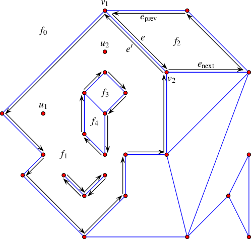
Figure 35.2 An arrangement of interior-disjoint line segments with some of the DCEL records that represent it. The unbounded face \( f_0\) has a single connected component that forms a hole inside it, and this hole comprises of several faces. The halfedge \( e\) is directed from its source vertex \( v_1\) to its target vertex \( v_2\). This edge, together with its twin \( e'\), correspond to a line segment that connects the points associated with \( v_1\) and \( v_2\) and separates the face \( f_1\) from \( f_2\). The predecessor \( e_{\rm prev}\) and successor \( e_{\rm next}\) of \( e\) are part of the chain that form the outer boundary of the face \( f_2\). The face \( f_1\) has a more complicated structure as it contains two holes in its interior: One hole consists of two adjacent faces \( f_3\) and \( f_4\), while the other hole comprises of two edges. \( f_1\) also contains two isolated vertices \( u_1\) and \( u_2\) in its interior.
One of the main components of the 2D Arrangements package is the Arrangement_2<Traits,Dcel> class template. An instance of this template is used to represent an arrangement embedded in the plane. The class template provides the interface needed to construct such arrangements, traverse them, and maintain them.
The design of the 2D Arrangements package is guided by two aspects of modularity as follows:
The latter separation is exhibited by the two template parameters of the Arrangement_2 class template; their description follows.
The Traits template-parameter should be substituted by a model of the ArrangementBasicTraits_2 concept and optionally additional geometry traits concepts. A model of the ArrangementBasicTraits_2 concept defines the types of \(x\)-monotone curves and two-dimensional points, namely ArrangementBasicTraits_2::X_monotone_curve_2 and ArrangementBasicTraits_2::Point_2, respectively, and supports basic geometric predicates on them. The instantiated traits class determines the family of planar curves that induce the arrangement.
In this section we always use Arr_non_caching_segment_traits_2 as our traits-class model in order to construct arrangements of line segments. In succeeding sections we also use Arr_segment_traits_2 as our traits-class model. These two traits trade computation time and storage space. The latter stores the underlying line of every segment of the arrangement to expedite certain operations on the arrangement segments. In Section Arrangements of Unbounded Curves we use Arr_linear_traits_2 to construct arrangements of linear curves (i.e., lines, rays, and line segments). The 2D Arrangements package contains several other traits classes that can handle other types of curves, such as polylines (continuous piecewise-linear curves), conic arcs, and arcs of rational functions. We exemplify the usage of these traits classes in Section The Geometry Traits.
Dcel template-parameter should be substituted by a class that models the ArrangementDcel concept, which is used to represent the topological layout of the arrangement. This parameter is substituted by Arr_default_dcel<Traits> by default, and we use this default value in this and in the following three sections. However, in many applications it is necessary to extend the DCEL features. This is done by substituting the Dcel parameter with a different type (typically, a different instance of the Arr_dcel<> class template); see Section Extending the DCEL for further explanations and examples. The function template print_arrangement_size() listed below, and defined in the header file Arr_print.h, prints out quantitative measures of a given arrangement. While in what follows it is used only by examples, it demonstrates well the use of the member functions number_of_vertices(), number_of_edges(), and number_of_faces(), which return the number of vertices, edges, and faces of an arrangement, respectively.
You can also obtain the number of halfedges of an arrangement using the member function number_of_halfedges(). Recall that the number of halfedges is always twice the number of edges.
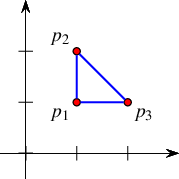
The simple program listed below constructs an arrangement of three connected line segments forming a triangle. It uses the Cartesian kernel with an integral-number type to instantiate the Arr_non_caching_segment_traits_2<Kernel> class template. The resulting arrangement consists of two faces, a bounded triangular face and the unbounded face. Constructing and maintaining arrangements using limited-precision numbers, such as int, works properly only under severe restrictions, which in many cases render the program not very useful. In this example, however, the points are far apart, and constructions of new geometric objects do not occur. Thus, it is safe to use int after all. The program constructs an arrangement induced by three line segments that are pairwise disjoint in their interior, prints out the number of faces, and ends. It uses the insert() free-function, which inserts the segments into the arrangement; see Section Free Functions. It uses the member function number_of_faces() to obtain the number of faces (two in this case). We give more elaborate examples in the rest of this chapter. The programs in those examples rely on computing with numbers of arbitrary precision, which guarantees robust execution and correct results.
The simplest and most fundamental arrangement operations are the various traversal methods, which allow users to systematically go over the relevant features of the arrangement at hand.
As mentioned above, the arrangement is represented as a DCEL, which stores three containers of vertices, halfedges and faces; thus, the Arrangement_2 class template supplies iterator types for these containers, respectively. For example, if arr is an Arrangement_2 object, the calls arr.vertices_begin() and arr.vertices_end() return iterators of the nested Vertex_iterator type that define the valid range of vertices of the arrangement arr. The value type of this iterator is Vertex. Moreover, the vertex-iterator type is convertible to Vertex_handle, which serves as a pointer to a vertex. As we show next, all functions related to arrangement features accept handle types as input parameters and return handle types as their output. See Chapter Handles and Circulators for more information on CGAL handles.
In addition to the iterators for arrangement vertices, halfedges, and faces, the arrangement class also provides an iterator for edges, namely Edge_iterator. The value type of this iterator is Halfedge, which is the same as the value type of Halfedge_iterator. The calls arr.edges_begin() and arr.edges_end() return iterators that define the valid range of arrangement edges. This range consists of half the number of halfedges of the arrangement, as every twin halfedges has one representative in this range.
All iterator, circulatorA circulator is used to traverse a circular list, such as the list of halfedges incident to a vertex. and handle types also have non-mutable (const) counterparts. These non-mutable iterator types are useful for traversing an arrangement with the promise to keep it unchanged. For example, the arrangement has a non-constant member function called Arrangement_on_surface_2::vertices_begin() that returns a Vertex_iterator object and another const member function that returns a Vertex_const_iterator object. In fact, all methods listed in this section that return an iterator, a circulator, or a handle have non-mutable counterparts. It should be noted that, for example, Vertex_handle can be readily converted into a Vertex_const_handle, but not the other way around.
Conversions of non-mutable handles to the corresponding mutable handles are nevertheless possible. They can be performed using the overloaded member function non_const_handle(). There are three variants that accept a non-mutable handle to a vertex, a halfedge, or a face, respectively. The call non_const_handle() can be issued only if the arrangement object arr is mutable; see, e.g., Section Point-Location Queries.
A vertex \(v\) of an arrangement induced by bounded curves is always associated with a geometric entity, namely with an Point_2 object, which can be obtained by v->point(), where v identifies a handle to \(v\).
The call v->is_isolated() determines whether the vertex \(v\) is isolated or not. Recall that the halfedges incident to a non-isolated vertex, namely, the halfedges that share a common target vertex, form a circular list around this vertex. The call v->incident_halfedges() returns a circulator of the nested type Halfedge_around_vertex_circulator that enables the traversal of this circular list around a given vertex \(v\) in a clockwise order. The value type of this circulator is Halfedge. By convention, the target of the halfedge is \(v\). The call v->degree() evaluates to the number of the halfedges incident to \(v\).
The function below prints all the halfedges incident to a given arrangement vertex (assuming that objects of the Point_2 type can be inserted into the standard output using the << operator). The arrangement type is the same as in the simple example above.
If \(v\) is an isolated vertex, the call v->face() can be used to obtain the face that contains \(v\).
A halfedge \(e\) of an arrangement induced by bounded curves is associated with an X_monotone_curve_2 object, which can be obtained by e->curve(), where e identifies a handle to \(e\).
The calls e->source() and e->target() return handles to the halfedge's source-vertex and target-vertex, respectively. You can obtain a handle to the twin halfedge using e->twin(). Note that from the definition of halfedges in the Dcel structure, the following invariants always hold:
e->curve() is equivalent to e->twin()->curve(), e->source() is equivalent to e->twin()->target(), and e->target() is equivalent to e->twin()->source(). Every halfedge has an incident face that lies to its left, which can be obtained by e->face(). Recall that a halfedge is always one link in a connected chain (CCB) of halfedges that share the same incident face. The e->prev() and e->next() calls return handles to the previous and next halfedges in the CCB, respectively.
As the CCB is a circular list of halfedges, it is only natural to traverse it using a circulator. Indeed e->ccb() returns an Ccb_halfedge_circulator object for traversing all halfedges along the connected component of \(e\). The value type of this circulator is Halfedge.
The function template print_ccb() listed below prints all \(x\)-monotone curves along a given CCB (assuming that objects of the Point_2 and the X_monotone_curve_2 types can be inserted into the standard output using the << operator).
An Arrangement_2 object arr that identifies an arrangement of bounded curves always has a single unbounded face. The call arr.unbounded_face() returns a handle to this face. Note that an empty arrangement contains nothing but the unbounded face.
Given a handle to a face \(f\), you can use the call f->is_unbounded() to determine whether the face \(f\) is unbounded. Bounded faces have an outer CCB, and the outer_ccb() method returns a circulator for the halfedges along this CCB. Note that the halfedges along this CCB wind in a counterclockwise order around the outer boundary of the face.
A face can also contain disconnected components in its interior, namely, holes and isolated vertices. You can access these components as follows:
You can obtain a pair of iterators of type Hole_iterator that define the range of holes inside a face \(f\) by calling f->holes_begin() and f->holes_end(). The value type of this iterator type is Ccb_halfedge_circulator, defining the CCB that winds in a clockwise order around a hole. The call f->number_of_holes() return the number of holes in \(f\).
The calls f->isolated_vertices_begin() and f->isolated_vertices_end() return iterators of type Isolated_vertex_iterator that define the range of isolated vertices inside the face \(f\). The value type of this iterator is Vertex.
The function print_face() listed below prints the outer and inner boundaries of a given face. It uses the function template print_ccb() listed above.
The function print_arrangement() listed below prints the features of a given arrangement. The file arr_print.h, which can be found under the examples folder, includes the definitions of this function, as well as the definitions of all other functions listed in this section. This concludes the preview of the various traversal methods.
In this section we review the various member functions of the Arrangement_2 class that allow users to modify the topological structure of the arrangement through the introduction of new edges or vertices, or the modification or removal of existing edges and vertices.
The arrangement member-functions that insert new \(x\)-monotone curves into the arrangement, thus enabling the construction of a two-dimensional surface subdivision, are rather specialized, as they assume that the interior of the inserted curve is disjoint from all existing arrangement vertices and edges, and in addition require apriori knowledge of the location of the inserted curve. Indeed, for most purposes it is more convenient to construct an arrangement using the free (global) insertion functions, which relax these restrictions. However, as these free functions are implemented in terms of the specialized insertion functions, we start by describing the fundamental functionality of the arrangement class, and describe the operation of the free functions in Section Free Functions.
The most trivial functions that allow users to modify the arrangement are the specialized functions for the insertion of an \(x\)-monotone curve the interior of which is disjoint from the interior of all other curves in the existing arrangement and does not contain any point of the arrangement. In addition, these functions require that the location of the curve in the arrangement be known.
The rather harsh restrictions on the inserted curves enable an efficient implementation. While inserting an \(x\)-monotone curve, the interior of which is disjoint from all curves in the existing arrangement, is quite straightforward, as we show next, (efficiently) inserting a curve that intersects with the curves already in the arrangement is much more complicated and requires the application of nontrivial geometric algorithms. The decoupling of the topological arrangement representation from the various algorithms that operate on it dictates that the general insertion operations be implemented as free functions that operate on the arrangement and the inserted curve(s); see Section Free Functions for more details and examples.

Figure 35.3 Illustrations of the various specialized insertion procedures. The inserted \(x\)-monotone curve is drawn as a dashed line, surrounded by two solid arrows that represent the pair of twin halfedges added to the DCEL. Existing vertices are shown as red discs, while new vertices are shown as blue discs. Existing halfedges that are affected by the insertion operations are drawn as dashed arrows. (a) Inserting a curve as a new hole inside the face \(f\). (b) Inserting a curve from an existing vertex \(u\) that corresponds to one of its endpoints. (c) Inserting an \(x\)-monotone curve, the endpoints of which correspond to existing vertices \(u_1\) and \(u_2\). In this case, the new pair of halfedges closes a new face \(f'\). The hole \(h_1\), which belonged to \(f\) before the insertion, becomes a hole in this new face.
When an \(x\)-monotone curve is inserted into an existing arrangement, such that the interior of this curve is disjoint from the interiors of all curves in the arrangement, only the following three scenarios are possible, depending on the status of the endpoints of the inserted curve:
Neither curve endpoints correspond to any existing arrangement vertex. In this case we have to create two new vertices that correspond to the curve endpoints, respectively, and connect them using a pair of twin halfedges. This halfedge pair forms a new hole inside the face that contains the curve in its interior.
Exactly one endpoint corresponds to an existing arrangement vertex. (We distinguish between a vertex that corresponds to the left endpoint of the inserted curve and a vertex that corresponds to its right endpoint.) In this case we have to create a new vertex that corresponds to the other endpoint of the curve and to connect the two vertices by a pair of twin halfedges that form an "antenna" emanating from the boundary of an existing connected component. (Note that if the existing vertex is isolated, we need to form a new hole inside the face that contains this vertex, essentially falling back to the handling of the previous case, naturally, skipping the creation of the existing vertex.)
Both endpoints correspond to existing arrangement vertices. In this case we connect these vertices using a pair of twin halfedges. (If one or both vertices are isolated, we fall back to the handling of the first or second case, respectively, naturally, skipping the creation of the existing vertices.) The two following subcases may occur:
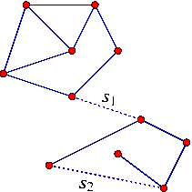
Two disconnected components are merged into a single connected component (as is the case with the segment \(s_1\) in the figure below).
A new face, which is split from an existing arrangement face, is created (as is the case with the segment \(s_2\) in the figure below). In this case we also have to examine the holes and isolated vertices in the existing face and move the relevant ones inside the new face.
The Arrangement_2 class offers insertion functions that perform the special insertion procedures listed above, namely, insert_in_face_interior(), insert_from_left_vertex(), insert_from_right_vertex() and insert_at_vertices(). The first function accepts an \(x\)-monotone curve \(c\) and an arrangement face \(f\) that contains this curve in its interior. The other functions accept an \(x\)-monotone curve \(c\) and handles to the existing vertices that correspond to the curve endpoint(s). Each of the four functions returns a handle to one of the twin halfedges that have been created; more precisely:
insert_in_face_interior(c, f) returns a handle to the halfedge directed from the left endpoint of \(c\) towards the vertex corresponding to its right endpoint.
insert_from_left_vertex(c, v) and insert_from_right_vertex(c, v) each returns a handle to the halfedge, the source of which is the vertex \(v\), and the target of which is the new vertex that has just been created.
insert_at_vertices(c, v1, v2) returns a handle to the halfedge directed from \(v_1\) to \(v_2\).
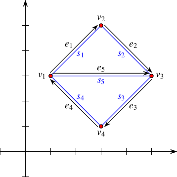
Figure 35.4 The arrangement of the line segments \(s_1, \ldots, s_5\) constructed in Arrangement_on_surface_2/edge_insertion.cpp. The arrows mark the direction of the halfedges returned from the various insertion functions.
The program below demonstrates the usage of the four specialized insertion functions. It creates an arrangement of five line segments \(s_1, \ldots, s_5\), as depicted in Figure 35.4. Notice that in all figures in the rest of this chapter the coordinate axes are drawn only for illustrative purposes and are not part of the arrangement. The first line segment \(s_1\) is inserted in the interior of the unbounded face, while the four succeeding line segments \(s_2, \ldots, s_5\) are inserted using the vertices created by the insertion of preceding segments. The arrows in the figure mark the direction of the halfedges \(e_1, \ldots, e_5\) returned from the insertion functions. The resulting arrangement consists of three faces, where the two bounded faces form together a hole in the unbounded face.
Two header files are included in the code in order to make this and the following examples more compact. The file arr_inexact_construction_segments.h is listed immediately after the program. The file arr_print.h is introduced in Section Traversing the Arrangement.
File Arrangement_on_surface_2/edge_insertion.cpp
The statements below define the types for arrangements of line segments common to all examples that do not construct new geometric objects. They are kept in the header file arr_inexact_construction_segments.h. In these examples the Traits parameter of the Arrangement_2<Traits, Dcel> class template is substituted by an instance of the Arr_non_caching_segment_traits_2<Kernel> class template. The Arr_non_caching_segment_traits_2 class template is instantiated with the predefined kernel that evaluates predicates in an exact manner, but constructs geometric objects in an inexact manner, as none of these examples construct new geometric objects. In the remaining examples the traits class-template is instantiated with a kernel that evaluates predicates and constructs geometric objects, both in an exact manner.
Isolated points are simpler geometric entities than curves, and indeed the member functions that manipulate them are easier to understand.
The call arr.insert_in_face_interior(p, f) inserts an isolated point \(p\), located in the interior of a given face \( f\), into the arrangement and returns a handle to the arrangement vertex associated with \(p\) it has created. Naturally, this function has a precondition that \(p\) is really an isolated point; namely it does not coincide with any existing arrangement vertex and does not lie on any edge. As mentioned in Section Traversing the Arrangement, it is possible to obtain the face containing an isolated vertex calling the member function Arrangement_on_surface_2::Vertex::face(). The member function Arrangement_on_surface_2::remove_isolated_vertex(Vertex_handle v) accepts a handle to an isolated vertex and removes it from the arrangement.
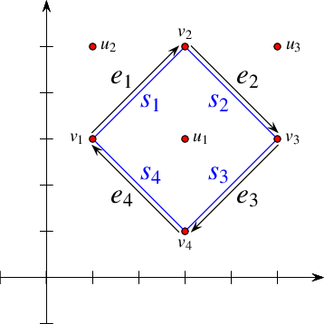
Figure 35.5 An arrangement of line segments containing three isolated vertices, as constructed in Arrangement_on_surface_2/isolated_vertices.cpp. The vertices \(u_2\) and \(u_3\) are eventually removed from the arrangement.
The following program demonstrates the usage of the arrangement member-functions for manipulating isolated vertices. It first inserts three isolated vertices, \(u_1\), \(u_2\), and \(u_3\), located inside the unbounded face of the arrangement. Then, it inserts four line segments \(s_1, \ldots, s_4\), that form a square hole inside the unbounded face (see Figure 35.4 for an illustration). Finally, it traverses the vertices and removes those isolated vertices that are still contained in the unbounded face ( \(u_2\) and \(u_3\) in this case):
File Arrangement_on_surface_2/isolated_vertices.cpp
While reading the previous subsection you learned how to insert new points that induce isolated vertices into the arrangement. You may wonder now how you can insert a new point that lies on an \(x\)-monotone curve that is associated with existing arrangement edge.
The introduction of a vertex, the geometric mapping of which is a point \(p\) that lies on an \(x\)-monotone curve, requires the splitting of the curve in its interior at \(p\). The two resulting subcurves induce two new edges, respectively. In general, the Arrangement_2 class template relies on the geometry traits to perform such a split. As a matter of fact, it relies on the geometry traits to perform all geometric operations. To insert a point \(p\) that lies on an \(x\)-monotone curve associated with an existing edge \(e\) into the arrangement \(\mathcal{A}\), you must first construct the two curves \(c_1\) and \(c_2\), which are the two subcurves that result from splitting the \(x\)-monotone curve associated with the edge \(e\) at \(p\). Then, you have to issue the call arr.split_edge(he, c1, c2), where arr identifies the arrangement \(\mathcal{A}\) and he is a handle to one of the two halfedges that represent the edge \(e\). The function splits the two halfedges that represent \(e\) into two pairs of halfedges, respectively. Two new halfedges are incident to the new vertex \(v\) associated with \(p\). The function returns a handle to the new halfedge, the source of which is the source vertex of the halfedge handled by he, and the target of which is the new vertex \(v\).
The reverse operation is also possible. Consider a vertex \(v\) of degree \(2\) that has two incident edges \(e_1\) and \(e_2\) associated with two curves \(c_1\) and \(c_2\), respectively, such that the union of \(c_1\) and \(c_2\) results in a single continuous \(x\)-monotone curve \(c\) of the type supported by the traits class in use. To merge the edges \(e_1\) and \(e_2\) into a single edge associated with the curve \(c\), essentially removing the vertex \(v\) from the arrangement identified by arr, you need to issue the call arr.merge_edge(he1,
he2, c), where he1 and he2 are handles to halfedges representing \(e_1\) and \(e_2\), respectively.
Finally, the call remove_edge(he) removes the edge \(e\) from the arrangement, where he is a handle to one of the two halfedges that represents \(e\). Note that this operation is the reverse of an insertion operation, so it may cause a connected component to split into two, or two faces to merge into one, or a hole to disappear. By default, if the removal of \(e\) causes one of its end vertices to become isolated, this vertex is removed as well. However, you can control this behavior and choose to keep the isolated vertices by supplying additional Boolean flags to remove_edge() indicating whether the source or the target vertices are to be removed should they become isolated.

Figure 35.6 The three steps of the example program Arrangement_on_surface_2/edge_manipulation.cpp. In Step (a) it constructs an arrangement of four line segments. In Step (b) the edges \(e_1\) and \(e_2\) are split, and the split points are connected with a new segment \(s\) that is inserted into the arrangement. This operation is undone in Step (c), where \(e\) is removed from the arrangement, rendering its end vertices \(u_1\) and \(u_2\) redundant. We therefore remove these vertices by merging their incident edges and go back to the arrangement depicted in (a).
The following example program shows how the edge-manipulation functions can be used. The program works in three steps, as demonstrated in Figure 35.5. Note that the program uses the fact that split_edge() returns one of the new halfedges (after the split) that has the same direction as the original halfedge (the first parameter of the function) and is directed towards the split point. Thus, it is easy to identify the vertices \(u_1\) and \(u_2\) associated with the split points.
File Arrangement_on_surface_2/edge_manipulation.cpp
The member functions modify_vertex() and modify_edge() modify the geometric mappings of existing features of the arrangement. The call arr.modify_vertex(v, p) accepts a handle to a vertex \(v\) and a reference to a point \(p\), and sets \(p\) to be the point associated with the vertex \(v\). The call arr.modify_edge(he,
c) accepts a handle to one of the two halfedges that represent an edge \(e\) and a reference to a curve \(c\), and sets \(c\) to be the \(x\)-monotone curve associated with \(e\). (Note that both halfedges are modified; that is, both expressions e->curve() and e->twin()->curve() evaluate to \(c\) after the modification.) These functions have preconditions that \(p\) is geometrically equivalent to v->point() and \(c\) is equivalent to e->curve(), respectively.Roughly speaking, two curves are equivalent iff they have the same graph. In Section The Basic Concept we give a formal definition of curves and curve equivalence. If these preconditions are not met, the corresponding operation may invalidate the structure of the arrangement. At first glance it may seem as if these two functions are of little use. However, you should keep in mind that there may be extraneous data (probably non-geometric) associated with the point objects or with the curve objects, as defined by the traits class. With these two functions you can modify this data; see more details in Section Data Decorators. In addition, you can use these functions to replace a geometric object (a point or a curve) with an equivalent object that has a more compact representation. For example, if we use some simple rational-number type to represent the point coordinates, we can replace the point \((\frac{20}{40},
\frac{99}{33})\) associated with some vertex \(v\) with an equivalent point with normalized coordinates, namely \((\frac{1}{2},
3)\).

|
Assume that the specialized insertion function |
The Arrangement_2 class provides advanced versions of the specialized insertion functions for a curve \(c\), namely, insert_from_left_vertex(c, he_pred) and insert_from_right_vertex(c, he_pred). These functions accept a halfedge \(e_{\mathrm{pred}}\) as specified above, instead of a handle to a vertex \(v\). They are more efficient, as they take constant time and do not perform any geometric operations. Thus, you should use them when the halfedge \(e_{\mathrm{pred}}\) is known. In cases where the vertex \(v\) is isolated or the predecessor halfedge for the newly inserted curve is not known, the simpler versions of these insertion functions should be used. Similarly, the member function insert_at_vertices() is overloaded with two additional versions as follows. One accepts two handles to the two predecessor halfedges around the two vertices \(v_1\) and \(v_2\), respectively, that correspond to the curve endpoints. The other one accepts a handle to one vertex and a handle to the predecessor halfedge around the other vertex.
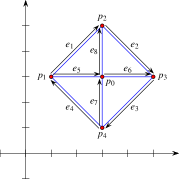
Figure 35.7 An arrangement of line segments, as constructed in Arrangement_on_surface_2/special_edge_insertion.cpp. Note that \(p_0\) is initially inserted as an isolated point and later on connected to the other four vertices.
The following program shows how to construct the arrangement depicted in Figure 35.7 using the specialized insertion functions that accept predecessor halfedges:
File Arrangement_on_surface_2/special_edge_insertion.cpp
It is possible to perform even more refined operations on an Arrangement_2 object given specific topological information. As most of these operations are very fragile and perform no precondition testing on their input in order to gain efficiency, they are not included in the public interface of the arrangement class. Instead, the Arr_accessor<Arrangement> class allows access to these internal arrangement operations; see more details in the Reference Manual.
One of the most useful query types defined on arrangements is the point-location query: Given a point, find the arrangement cell that contains it. Typically, the result of a point-location query is one of the arrangement faces, but in degenerate situations the query point can lie on an edge, or it may coincide with a vertex.
Point-location queries are common in many applications, and also play an important role in the incremental construction of arrangements (and more specifically in the free insertion-functions described in Section Free Functions). Therefore, it is crucial to have the ability to answer such queries effectively.
Recall that the arrangement representation is decoupled from the geometric algorithms that operate on it. Thus, the Arrangement_2 class template does not support point-location queries directly. Instead, the 2D Arrangements package provides a set of class templates that are capable of answering such queries; all are models of the concept ArrangementPointLocation_2. Each model employs a different algorithm or strategy for answering queries. A model of this concept must define the locate() member function, which accepts an input query-point and returns a polymorphic object representing the arrangement cell that contains this point. The returned object is of type Arr_point_location_result<Arrangement_2>::Type, which is a discriminated union container of the bounded types Vertex_const_handle, Halfedge_const_handle, or Face_const_handle. Depending on whether the query point is located inside a face, lies on an edge, or coincides with a vertex, the appropriate handle can be obtained with value retrieval by std::get as demonstrated in the example below.
Note that the handles returned by the locate() functions are non-mutable (const). If necessary, such handles may be cast to mutable handles using the Arrangement_on_surface_2::non_const_handle() methods.
An object pl of any point-location class must be attached to an Arrangement_2 object arr before it is used to answer point-location queries on arr. This attachment can be performed when pl is constructed or at a later time using the pl.init(arr) call.
The function template locate_point() listed below accepts a point-location object, the type of which is a model of the ArrangementPointLocation_2 concept, and a query point. The function template issues a point-location query for the given point, and prints out the result. It is defined in the header file point_location_utils.h.
The function template locate_point() calls an instance of the function template print_point_location(), which inserts the result of the query into the standard output-stream. It is listed below, and defined in the header file point_location_utils.h. Observe how the function std::get() is used to cast the resulting object into a handle to an arrangement feature. The point-location object pl is assumed to be already attached to an arrangement.
Each of the various point-location class templates employs a different algorithm or strategyThe term strategy is borrowed from the design-pattern taxonomy [7], Chapter 5. A strategy provides the means to define a family of algorithms, each implemented by a separate class. All classes that implement the various algorithms are made interchangeable, letting the algorithm in use vary according to the user choice. for answering queries:
Arr_naive_point_location<Arrangement> employs the naive strategy. It locates the query point naively, exhaustively scanning all arrangement cells.
Arr_walk_along_line_point_location<Arrangement> employs the walk-along-a-line (or walk for short) strategy. It simulates a traversal, in reverse order, along an imaginary vertical ray emanating from the query point. It starts from the unbounded face of the arrangement and moves downward toward the query point until it locates the arrangement cell containing it.
Arr_landmarks_point_location<Arrangement,Generator> uses a set of landmark points, the location of which in the arrangement is known. It employs the landmark strategy. Given a query point, it uses a nearest-neighbor search-structure (a Kd-tree is used by default) to find the nearest landmark, and then traverses the straight-line segment connecting this landmark to the query point.
There are various ways to select the landmark set in the arrangement. The selection is governed by the Generator template parameter. The default generator class, namely Arr_landmarks_vertices_generator, selects all the vertices of the attached arrangement as landmarks. Additional generators that select the set in other ways, such as by sampling random points or choosing points on a grid, are also available; see the Reference Manual for more details.
The landmark strategy requires that the type of the attached arrangement be an instance of the Arrangement_2<Traits,Dcel> class template, where the Traits parameter is substituted by a geometry-traits class that models the ArrangementLandmarkTraits_2 concept, which refines the basic ArrangementBasicTraits_2 concept; see Section The Landmark Concept for details. Most traits classes included in the 2D Arrangements package are models of this refined concept.
Arr_trapezoid_ric_point_location<Arrangement> implements an improved variant of Mulmuley's point-location algorithm [11]; see also [5], Chapter 6. The (expected) query-time is logarithmic in the size of the arrangement. The arrangement faces are decomposed into simpler cells each of constant complexity, known as pseudo trapezoids, and a search structure (a directed acyclic graph) is constructed on top of these cells, facilitating the search of the pseudo trapezoid (hence the arrangement cell) containing a query point in expected logarithmic time. The trapezoidal map and the search structure are built by a randomized incremental construction algorithm (RIC).
Arr_triangulation_point_location<Arrangement> uses a constrained triangulation, provided by the 2D Triangulations package, as a search structure. Every time the arrangement is modified the constrained triangulation search-structure is reconstructed from scratch, where the edges of the arrangement are set to be the constrained edges of the triangulation. This strategy is inefficient (especially when the number of modifications applied to the arrangement is high) and provided only for educational purposes.
The first two strategies do not require any extra data. The class templates that implement them store a pointer to an arrangement object and operate directly on it. Attaching such point-location objects to an existing arrangement has virtually no running-time cost at all, but the query time is linear in the size of the arrangement (the performance of the walk strategy is much better in practice, but its worst-case performance is linear). Using these strategies is therefore recommended only when a relatively small number of point-location queries are issued by the application, or when the arrangement is constantly changing (That is, changes in the arrangement structure are more frequent than point-location queries). On the other hand, the landmark and the trapezoid RIC strategies require auxiliary data structures on top of the arrangement structure, which they need to construct once they are attached to an arrangement object and need to keep up-to-date as this arrangement changes.
As mentioned above, the triangulation strategy is provided only for educational purposes, and thus we do not elaborate on this strategy. The data structure needed by the landmark and the trapezoidal map RIC strategies can be constructed in \(O(N \log N)\) time, where \(N\) is the overall number of edges in the arrangement, but the constant hidden in the \(O(~)\) notation for the trapezoidal map RIC strategy is much larger. Thus, construction needed by the landmark algorithm is in practice significantly faster than the construction needed by the trapezoidal map RIC strategy. In addition, although both resulting data structures are asymptotically linear in size, the actual amount of memory consumed by the landmark algorithm is typically smaller than to the amount used by the trapezoidal map RIC algorithm, due to the space-efficient Kd-tree used by the landmark algorithm as the nearest-neighbor search-structure. The trapezoidal map RIC algorithm has expected logarithmic query time, while the query time for the landmark algorithm may be as large as linear. In practice however, the query times of both strategies are competitive. For a detailed experimental comparison see [9].
Updating the auxiliary data structures of the trapezoidal map RIC algorithm is done very efficiently. On the other hand, updating the nearest-neighbor search-structure of the landmark algorithm may consume significant time when the arrangement changes frequently, especially when a Kd-tree is used, as it must be rebuilt each time the arrangement changes. It is therefore recommended that the Arr_landmarks_point_location class template be used when the application frequently issues point-location queries on an arrangement that only seldom changes. If the arrangement is more dynamic and is frequently going through changes, the Arr_trapezoid_ric_point_location class template should be the selected point-location strategy.
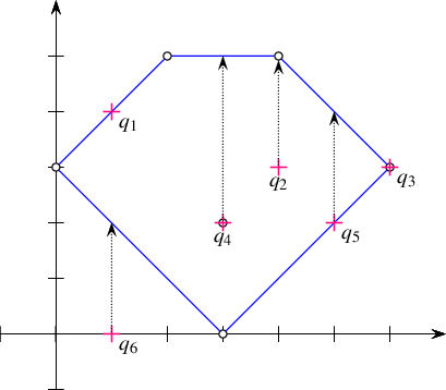
Figure 35.8 The arrangement of line segments, as constructed in Arrangement_on_surface_2/point_location.cpp, Arrangement_on_surface_2/vertical_ray_shooting.cpp, and Arrangement_on_surface_2/batched_point_location.cpp. The arrangement vertices are drawn as small rings, while the query points \(q_1, \ldots, q_6\) are drawn as crosses.
The program listed below constructs a simple arrangement of five line segments that form a pentagonal face, with a single isolated vertex in its interior, as depicted in Figure 35.8. Notice that we use the same arrangement structure in the next three example programs. The arrangement construction is performed by the function construct_segment_arr() defined in the header file point_location_utils.h. (Its listing is omitted here.) The program employs the naive and the landmark strategies to issue several point-location queries on this arrangement.
File Arrangement_on_surface_2/point_location.cpp
Note that the program uses the locate_point() function template to locate a point and nicely print the result of each query; see code example in Section Point-Location Queries.
Another query frequently issued on arrangements is the vertical ray-shooting query: Given a query point, which arrangement cell is encounter by a vertical ray shot upward (or downward) from this point? In the general case the ray hits an edge, but it is possible that it hits a vertex, or that the arrangement does not have any vertex or edge lying directly above (or below) the query point.
All point-location classes listed in the previous section are also models of the ArrangementVerticalRayShoot_2 concept. That is, they all have member functions called ray_shoot_up(q) and ray_shoot_down(q) that accept a query point \(q\). These functions output a polymorphic object of type Arr_point_location_result<Arrangement_2>::Type, which is a discriminated union container of the bounded types Vertex_const_handle, Halfedge_const_handle, or Face_const_handle. The latter type is used for the unbounded face of the arrangement, in case there is no edge or vertex lying directly above (or below) \(q\).
The function template vertical_ray_shooting_query() listed below accepts a vertical ray-shooting object, the type of which models the ArrangementVerticalRayShoot_2 concept. It exports the result of the upward vertical ray-shooting operation from a given query point to the standard output-stream. The ray-shooting object vrs is assumed to be already attached to an arrangement. The function template is defined in the header file point_location_utils.h.
The program below uses the function template listed above to perform vertical ray-shooting queries on an arrangement. The arrangement and the query points are exactly the same as in Arrangement_on_surface_2/point_location.cpp; see Figure 35.8.
File Arrangement_on_surface_2/vertical_ray_shooting.cpp
Suppose that at a given moment our application has to issue a relatively large number \(m\) of point-location queries on a specific arrangement object. Naturally, It is possible to define a point-location object and use it to issue separate queries on the arrangement. However, as explained in Section Point-Location Queries choosing a simple point-location strategy (either the naive or the walk strategy) means inefficient queries, while the more sophisticated strategies need to construct auxiliary structures that incur considerable overhead in running time.
Alternatively, the 2D Arrangement package includes a free locate() function that accepts an arrangement and a range of query points as its input and sweeps through the arrangement to locate all query points in one pass. The function outputs the query results as pairs, where each pair consists of a query point and a discriminated union container, which represents the cell containing the point; see Section Point-Location Queries. The output pairs are sorted in increasing \(xy\)-lexicographical order of the query point.
The batched point-location operation is carried out by sweeping the arrangement. Thus, it takes \(O((m+N)\log{(m+N)})\) time, where \(N\) is the number of edges in the arrangement. Issuing separate queries exploiting a point-location strategy with logarithmic query time per query, such as the trapezoidal map RIC strategy (see Section Choosing a Point-Location Strategy), is asymptotically more efficient. However, experiments show that when the number \(m\) of point-location queries is of the same order of magnitude as \(N\), the batched point-location operation is more efficient in practice. One of the reasons for the inferior performance of the alternative (asymptotically faster) procedures is the necessity to construct and maintain complex additional data structures.
The program below issues a batched point-location query, which is essentially equivalent to the six separate queries performed in Arrangement_on_surface_2/point_location.cpp; see Section Point-Location Queries.
File Arrangement_on_surface_2/batched_point_location.cpp
The Arrangement_on_surface_2 class template is used to represent subdivisions of two-dimensional surfaces induced by curves that lie on such surfaces. Its interface is minimal in the sense that the member functions hardly perform any geometric operations. In this section we explain how to utilize the free functions that enhance that set of operations on arrangements. The implementation of these operations typically require non-trivial geometric algorithms, and occasionally incurs additional requirements on the geometry traits class; the implementation of many of the operations is based on two frameworks, namely the surface sweep and the zone construction. These operations accepts \(x\)-monotone curves; thus, the geometry-traits class used by the arrangements passed as input to, or obtained as output from, these operations must be a model of the ArrangementXMonotoneTraits_2 concept; see Section The Geometry Traits for the precise definition of this concept. It defines the minimal set of geometric primitives, among other things, required to perform the algorithms of the surface-sweep and zone-construction frameworks.
Given an arrangement of curves \(\mathcal{A} = \mathcal{A}(\mathcal{C})\) embedded in a two-dimensional surface, the zone of an additional curve \(\gamma \notin \mathcal{C}\) in \(\mathcal{A}\) is the union of the features of \(\mathcal{A}\), whose closure is intersected by \(\gamma\). The complexity of the zone is defined as the sum of the complexities of its constituents. (Notice that some vertices are counted multiple times.) The zone of a curve \(\gamma\) is computed by locating the left endpoint of \(\gamma\) in the arrangement and then "walking"' along the curve towards the right endpoint, keeping track of the vertices, edges, and faces crossed on the way. The 2D Arrangements package offers a generic implementation of an algorithm that computes the zone. It is used to implement a set of operations that incrementally construct arrangements induced by sets of curves that lie in two-dimensional surfaces. For simplicity, however, we continue to consider arrangements embedded in the plane.
Section The Arrangement Class Template explains how to construct arrangements of \(x\)-monotone curves that are pairwise disjoint in their interior when the location of the segment endpoints in the arrangement is known. Here we relax this constraint, and allow the location of the inserted \(x\)-monotone curve endpoints to be unknown at the time of insertion.
We retain, for the moment, the requirement that the interior of the inserted curve is disjoint from all existing arrangement edges and vertices.
The call insert_non_intersecting_curve(arr, c, pl) inserts the \(x\)-monotone curve \(c\) into the arrangement arr, with the precondition that the interior of \(c\) is disjoint from all existing edges and vertices of arr. The third argument pl is a point-location object attached to the arrangement; it is used to locate both endpoints of \(c\) in the arrangement. Each endpoint is expected to either coincide with an existing vertex or lie inside a face. It is possible to invoke one of the specialized insertion functions (see Section The Arrangement Class Template), based on the query results, and insert \(c\) at its proper location.The CGAL::insert_non_intersecting_curve<>() function template, as all other functions reviewed in this section, is parameterized by an arrangement type and a point-location type (The latter must be substituted by a model of the ArrangementPointLocation_2 concept). The insertion operation thus hardly requires any geometric operations on top of the ones needed to answer the point-location queries. Moreover, it is sufficient that the traits class that substitutes the Traits template parameter of the Arrangement_2<Traits,Dcel> class template when the latter is instantiated models the concept ArrangementBasicTraits_2 concept (and the concept ArrangementLandmarkTraits_2 if the landmark point-location strategy is used), and does not have to support the computation of intersection points between curves. This implies that using a kernel that provides exact geometric predicates, but potentially inexact geometric constructions due to round-off errors, is still sufficient.
The free-function template CGAL::insert_non_intersecting_curve<>(arr, c, pl) is overloaded. There is a variant that instead of accepting a user-defined point-location object, it constructs a local object of the walk point-location type, namely, an instance of the Arr_walk_along_line_point_location class template, and uses it to insert the curve.
The time it takes to insert a curve \(c\) using the insert_non_intersecting_curve() function template is the sum of the time is takes to locate the two endpoints of \(c\) and the time is takes to find the exact place for the new two halfedges mapped to \(c\) in the circular list of halfedges incident to the two vertices mapped to the endpoints of \(c\), respectively. This makes the function relatively efficient; however, its preconditions on the input curves are still rather restricting. Let us assume that the traits class that substitutes the Traits template parameter of the Arrangement_2<Traits,Dcel> class template models the refined ArrangementXMonotoneTraits_2 concept and supports curve intersection computations; see Section The Geometry Traits for the exact details. Given an \(x\)-monotone curve, it is sufficient to locate its left endpoint in the arrangement and to trace its zone (see Section The Zone Construction Algorithm) until the right endpoint is reached. Each time the new curve \(c\) crosses an existing vertex or edge, the curve is split into subcurves (in the latter case, we have to split the curve associated with the existing halfedge as well) and new edges are associated with the resulting subcurves. Recall that an edge is represented by a pair of twin halfedges, so we split it into two halfedge pairs.
The call insert(arr, c, pl) performs this insertion operation. The CGAL::insert<>() function template accepts an \(x\)-monotone curve \(c\), which may intersect some of the curves already in the arrangement arr, and inserts it into the arrangement by computing its zone. Users may supply a point-location object pl or use the default walk point-location strategy (namely, the variant CGAL::insert<>(arr, c) is also available). The running-time of this insertion function is proportional to the complexity of the zone of the curve \(c\).
In some cases users may have a prior knowledge of the location of the left endpoint of the \(x\)-monotone curve \(c\) they wish to insert, so they can perform the insertion without issuing any point-location queries. This can be done by calling the free function template CGAL::insert<>(arr, c, obj), where obj is a polymorphic object of type Arr_point_location_result<Arrangement_2>::Type that represents the location of \(c\)s left endpoint in the arrangement. It is a discriminated union container of the bounded types Vertex_const_handle, Halfedge_const_handle, or Face_const_handle; see also Section Point-Location Queries.
So far, all the examples have constructed arrangements of line segments, where the Arrangement_2 template was instantiated with an instance of the Arr_segment_traits_2 class template. In this case, the restriction that CGAL::insert<>() requires an \(x\)-monotone is irrelevant, as all line segments are \(x\)-monotone. (Note that we always deal with weakly \(x\)-monotone curves, and we consider vertical line-segments to be weakly \(x\)-monotone).
Consider an arrangement of circles. A circle is obviously not \(x\)-monotone, so CGAL::insert<>() cannot be used in this case.A key operation performed by CGAL::insert<>() is to locate the left endpoint of the curve in the arrangement. A circle, however, does not have any endpoints! , it is necessary to subdivide each circle into two \(x\)-monotone circular arcs, namely, its upper half and its lower half, and to insert the two individual \(x\)-monotone arcs.
The free function template CGAL::insert<>() is overloaded. It is possible to another version of this function and pass a curve that is not necessarily \(x\)-monotone, but this is subject to an important condition. Consider the call insert(arr, c,
pl), where \(c\) is not necessarily \(x\)-monotone. In this case the type of arr must be an instance of the Arrangement_2<Traits, Dcel> class template, where the Traits template parameter is substituted by a traits class that models the concept ArrangementTraits_2, which refines the ArrangementXMonotoneTraits_2 concept. It has to define an additional Curve_2 type, which may differ from the X_monotone_curve_2 type. It also has to support the subdivision of curves of this new type into \(x\)-monotone curves and possibly singular points; see the exact details in Section The Geometry Traits. The CGAL::insert<>(arr, c, pl) function performs the insertion of the curve \(c\) that does not need to be \(x\)-monotone, into the arrangement by subdividing it into \(x\)-monotone subcurves and inserting all individual \(x\)-monotone subcurves. Users may supply a point-location object pl, or use the default walk point-location strategy by calling CGAL::insert<>(arr, c).
The Arrangement_2 class template has a member function that inserts a point as an isolated vertex in a given face. The free function template CGAL::insert_point<>(arr, p, pl) inserts a vertex that corresponds to the point \(p\) into arr at an arbitrary location. It uses the point-location object pl to locate the point in the arrangement (by default, the walk point-location strategy is used), and acts according to the result as follows:
If \(p\) is located inside a face, it is inserted as an isolated vertex inside this face.
If \(p\) lies on an edge, the edge is split to create a vertex associated with \(p\).
In all cases, the function returns a handle to the vertex associated with \(p\).
The type of arr must be and instance of the Arrangement_2 class template instantiated with a traits class that models the ArrangementXMonotoneTraits_2 concept, as the insertion operation may involve the splitting of curves.
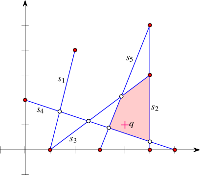
Figure 35.9 An arrangement of five intersecting line segments, as constructed in Arrangement_on_surface_2/incremental_insertion.cpp and Arrangement_on_surface_2/aggregated_insertion.cpp. The segment endpoints are marked by black disks and the arrangement vertices that correspond to intersection points are marked by circles. The query point \(q\) is marked with a cross and the face that contains it is shaded.
The program below constructs an arrangement of five intersecting line-segments \(s_1, \ldots, s_5\). It is known that \(s_1\) and \(s_2\) do not intersect, so CGAL::insert_non_intersecting_curve<>() is used to insert them into the empty arrangement. The rest of the segments are inserted using CGAL::insert<>(). Using a kernel that constructs geometric objects in an inexact manner (due to round-off errors) may yield a program that computes incorrect results and crashes from time to time. This is avoided by using a kernel that provides exact geometric-object constructions as well as exact geometric-predicate evaluations. The header file arr_exact_construction_segments.h, just like the header file arr_inexact_construction_segments.h, contains the definitions for arrangements of line segments. Unlike the latter, it uses a kernel suitable for arrangements induced by curves that intersect each other, namely a kernel that is exact always. Note that we alternately use the naive point-location strategy, given explicitly to the insertion functions, and the default walk point-location strategy.
The resulting arrangement is depicted in Figure 35.9, where the vertices that correspond to segment endpoints are drawn as dark discs, and the vertices that correspond to intersection points are drawn as circles. It consists of 13 vertices, 16 edges, and 5 faces. We also perform a point-location query on the resulting arrangement. The query point \(q\) is drawn as a plus sign. The face that contains it is drawn with a shaded texture. The program calls an instance of the function template print_arrangement_size(), which prints quantitative measures of the arrangement; see code example for its listing in Section The Arrangement Class Template.
File Arrangement_on_surface_2/incremental_insertion.cpp
In this section we have described so far free functions that insert curves and points into a given arrangement. Now we describe functions that do not change the arrangement at all; nevertheless, they are closely related to the incremental insertion functions, as they also use the zone framework.
The free function template CGAL::do_intersect<>(arr, c, pl) checks whether the given query curve \(c\) intersects the curves and points of an existing arrangement arr. If \(c\) is not \(x\)-monotone (that is, it is of type Curve_2) the curve is subdivided into \(x\)-monotone subcurves and isolated points. Each \(x\)-monotone curve (or point) is checked for intersection in turn using the zone framework. For points we simply apply point-location. Given an \(x\)-monotone curve, first its left endpoint is located; then, its zone is computed starting from its left endpoint location. The zone computation terminates when an intersection with an arrangement curve or point is found or when the right endpoint is reached. A given point-location object is used for locating the left endpoint of the curve in the existing arrangement. There is a variant that instead of accepting a user-defined point-location object, it constructs a local object of the walk point-location type, namely, an instance of the Arr_walk_along_line_point_location class template, and uses it to locate the endpoint. If the given curve is \(x\)-monotone then the traits type must model the ArrangementXMonotoneTraits_2 concept. If the curve is not \(x\)-monotone then the traits type must model the ArrangementTraits_2 concept.
The CGAL::zone<>(arr, c, oi, pl) function template computes the zone of a given \(x\)-monotone curve in a given arrangement. More precisely, it outputs all the arrangement cells (namely, vertices, edges, and faces) that the input \(x\)-monotone curve \(C\) intersects in the order they are discovered when traversing the curve from left to right. The function uses a given point-location object to locate the left endpoint of the given curve. There is a variant that instead of accepting a user-defined point-location object, it constructs a local object of the walk point-location type, namely, an instance of the Arr_walk_along_line_point_location class template, and uses it to locate the endpoint. The traits type must model the ArrangementXMonotoneTraits_2 concept.
The famous plane-sweep algorithm introduced by Bentley and Ottmann was originally formulated for sets of line segments in the plane. The 2D Intersection of Curves package offers a generic implementation of a generalized version of the original plane-sweep algorithm. It (i) operates in two-dimensional surfaces (not restricted to the plane), (ii) accepts various families of \(x\)-monotone curves (not only line segments), and (iii) handles overlaps. (Observe that the original algorithm did not handle overlaps. Handling overlaps is difficult, especially for polyline, as two polylines may overlap in more then one connected component.) The generic implementation serves as the foundation of a family of concrete operations described in the rest of this section, such as aggregately constructing an arrangement induced by a set of curves that lie in a two-dimensional surface and outputting the overlay of two arrangements.
Given a set of \(n\) input curves, you can insert the curves in the set into an arrangement incrementally one by one. However, the 2D Arrangements package also provides a couple of free (overloaded) functions that aggregately insert a range of curves into an arrangement using the surface-Sweep framework.
CGAL::insert_non_intersecting_curves<>(arr, begin, end) inserts a range of \(x\)-monotone curves given by the range [begin, end) into an arrangement arr. The \(x\)-monotone curves should be pairwise disjoint in their interior and also interior-disjoint from all existing curves and points of arr.
insert(arr, begin, end) operates on a range of \(x\)-monotone curves that may intersect one another.
We distinguish between two cases: (i) The given arrangement arr is empty (has only an unbounded face), so it must be construct from scratch. (ii) The given arrangement arr is not empty.
In the first case, we sweep over the input curves, compute their intersection points, and construct the DCEL that represents their arrangement. This process is performed in \(O((n + k)\log n)\) time, where \(k\) is the total number of intersection points. The running time is asymptotically better than the time needed for incremental insertion if the arrangement is relatively sparse (when \(k\) is \(O(\frac{n^2}{\log n})\)), but it is recommended that this aggregate construction process be used even for dense arrangements, since the plane-sweep algorithm performs fewer geometric operations compared to the incremental insertion algorithms, and hence typically runs much faster in practice.
Another important advantage of the aggregated insertion functions is that they do not issue point-location queries. Thus, no point-location object needs to be attached to the arrangement. As explained in Section Point-Location Queries, there is a trade-off between construction time and query time in each of the point-location strategies, which affects the running times of the incremental insertion process. Naturally, this trade-off is absent in the case of aggregated insertion.
The example below shows how to construct the same arrangement of five line segments built incrementally in Arrangement_on_surface_2/incremental_insertion.cpp depicted in Figure 35.9 using the aggregate insertion function insert(). Note that no point-location object needs to be defined and attached to the arrangement.
File Arrangement_on_surface_2/aggregated_insertion.cpp
Next we handle the case where we have to insert a set of \(n\) curves into an existing arrangement. Let \(N\) denote the number of edges in the arrangement. If \(n\) is very small compared to \(N\) (in theory, we would say that if \(n = o(\sqrt{N})\)), we insert the curves one by one. For larger input sets, we use the aggregate insertion procedures.
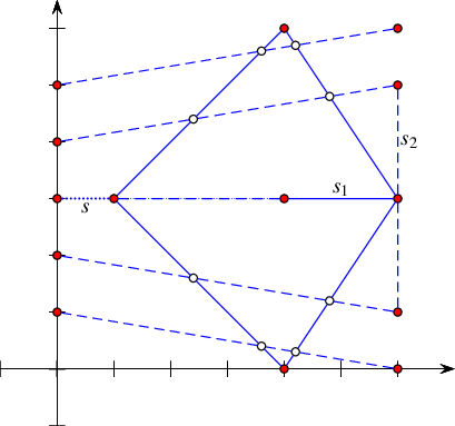
Figure 35.10 An arrangement of intersecting line segments, as constructed in Arrangement_on_surface_2/global_insertion.cpp. The segments of \(\mathcal{S}_1\) are drawn in solid lines and the segments of \(\mathcal{S}_2\) are drawn in dark dashed lines. Note that the segment \( s\) (light dashed line) overlaps one of the segments in \(\mathcal{S}_1\).
The program below aggregately construct an arrangement of a set \(\mathcal{S}_1\) containing five line segments (drawn as solid lines). Then, it inserts a single segment \(s\) (drawn as a dotted line) using the incremental insertion function. Finally, it adds a set \(\mathcal{S}_2\) with five more line segments (drawn as dashed lines) in an aggregate fashion. Notice that the line segments of \(\mathcal{S}_1\) are pairwise interior-disjoint, so insert_non_intersecting_curves() is safely used. \(\mathcal{S}_2\) also contains pairwise interior-disjoint segments, but as they intersect the existing arrangement, insert() must be used to insert them. Also note that the single segment \(s\) inserted incrementally partially overlaps an existing arrangement curve; the overlapped portion is drawn as a dash-dotted line.
File Arrangement_on_surface_2/global_insertion.cpp
We summarize the three levels of arrangement types based on curve monotonicity and intersection properties in the table below. The three levels, starting from the most restrictive, are (i) \(x\)-monotone curves that are pairwise disjoint in their interior, (ii) \(x\)-monotone curves (which are possibly intersecting one another), and (iii) general curves. We list the single-curve insertion functions.
| Type of Curves | Geometry-Traits Concept | Insertion Function |
|---|---|---|
| \(x\)-monotone and pairwise disjoint | ArrangementBasicTraits_2 or ArrangementLandmarkTraits_2 | CGAL::insert_non_intersecting_curve<>() |
| \(x\)-monotone | ArrangementXMonotoneTraits_2 | CGAL::insert<>() |
| general | ArrangementTraits_2 | CGAL::insert<>() |
The insertion function template insert() is overloaded to (i) incrementally insert a single \(x\)-monotone curve, (ii) incrementally insert a single general curve, (iii) aggregately insert a set of \(x\)-monotone curves, and (iv) aggregately insert a set of general curves. The CGAL::insert_non_intersecting_curves<>() function template aggregately inserts a set of \(x\)-monotone pairwise interior-disjoint curves into an arrangement.
The free functions remove_vertex() and remove_edge() handle the removal of vertices and edges from an arrangement, respectively. The difference between these functions and the corresponding member functions of the Arrangement_2 class template (see Section Manipulating Isolated Vertices and Section Manipulating Halfedges) has to do with the ability to merge two curves associated with adjacent edges to form a single curve associated with a single edge. An attempt to remove a vertex or an edge from an arrangement object arr using the free functions above requires that the traits class used to instantiate the arrangement type of arr models the concept ArrangementXMonotoneTraits_2, which refines the ArrangementBasicTraits_2 concept; see Section The Geometry Traits.
The function template CGAL::remove_vertex<>(arr, v) removes the vertex \(v\) from the given arrangement arr, where \(v\) is either an isolated vertex or is a redundant vertex. Namely, it has exactly two incident edges that are associated with two curves that can be merged to form a single \(x\)-monotone curve. If neither of the two cases apply, the function returns an indication that it has failed to remove the vertex.
The function CGAL::remove_edge<>(arr, e) removes the edge \(e\) from the arrangement by simply calling arr.remove_edge(e); see Section Modifying the Arrangement. In addition, if either of the end vertices of \(e\) becomes isolated or redundant after the removal of the edge, it is removed as well.
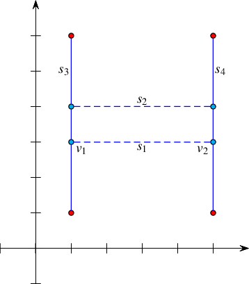
The following example demonstrates the usage of the free removal functions. It creates an arrangement of four line segment \(s_1, \ldots, s_4\) forming an H-shape with two horizontal edges induced by \(s_1\) and \(s_2\) (drawn as dashed lines). Then it removes the two horizontal edges and clears all redundant vertices (drawn as lightly shaded discs), such that the final arrangement consists of just two edges associated with the vertical line segments \(s_3\) and \(s_4\).
File Arrangement_on_surface_2/global_removal.cpp
As you have already seen, an arrangement face may have a fairly complicated structure; its outer boundary may be very large, and it may contain numerous holes. For many practical applications, it is more convenient to analyze the faces by decomposing each into a finite number of cells (preferably convex when dealing with arrangements of linear curves) of constant complexity. Vertical decomposition is a generic way to achieve such a simplification of the arrangement.
Given an arrangement, we consider each arrangement vertex \(v\), and locate the feature lying vertically below the vertex and the feature lying vertically above it, or the unbounded face in case there is no such feature. (Such a feature is also the result of the vertical ray-shooting operation from the vertex \(v\), as described in Section Vertical Ray Shooting.) It is now possible to construct two vertical segments connecting \(v\) to the feature above it and to the feature below it, possibly extending the vertical segments to infinity. The collection of the vertical segments and rays computed for all arrangement vertices induces a subdivision of the arrangement into simple cells. There are two types of bounded two-dimensional cells, as follows:
Cells whose outer boundaries comprise four edges, of which two originate from the original arrangement and the other two are vertical.
Cells whose outer boundaries comprise three edges, of which two originate from the original arrangement and intersect at a common vertex and the remaining one is vertical.
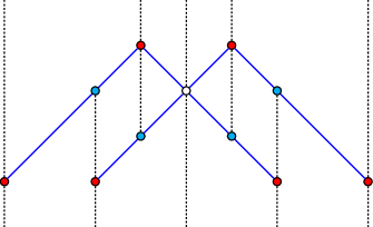
Figure 35.11 An arrangement of four line segments and its vertical decomposition into pseudo trapezoids, as constructed in Arrangement_on_surface_2/bounded_vertical_decomposition.cpp. The segments of the arrangement are drawn in solid blue lines and the segments of the vertical decomposition are drawn in dark dotted lines.
In the case of an arrangement of line segments, two-dimensional cells of the former type are trapezoids (as they have a pair of parallel vertical edges), while two-dimensional cells of the latter type are triangles, which can be viewed as degenerate trapezoids. The unbounded cells can be similarly categorized into two types. Observe that the boundary of an unbounded cell contains only one original edge or none and it may contain only non-vertical edges. The resulting cells are therefore referred to as pseudo trapezoids. The Figure 35.11 depicts the vertical decomposition of an arrangement induced by four line segments, as constructed in Arrangement_on_surface_2/bounded_vertical_decomposition.cpp and listed below. The decomposition consists of 14 pseudo trapezoids, out of which two are bounded triangles, two are bounded trapezoids, and 10 are unbounded trapezoids.
The function template decompose() accepts an arrangement \(\mathcal{A}\) and outputs for each vertex \(v\) of \(\mathcal{A}\) a pair of features—one that directly lies below \(v\) and another that directly lies above \(v\). It is implemented as a plane-sweep algorithm, which aggregately computes the set of pairs of features. Let \(v\) be a vertex of \(\mathcal{A}\). The feature above (respectively below) \(v\) may be one of the following:
Another vertex \(u\) having the same \(x\)-coordinate as \(v\).
An arrangement edge associated with an \(x\)-monotone curve that contains \(v\) in its \(x\)-range.
An unbounded face in case \(v\) is incident to an unbounded face, and there is no curve lying above (respectively below) it.
An empty object, in case \(v\) is the lower (respectively upper) endpoint of a vertical edge in the arrangement.
File Arrangement_on_surface_2/bounded_vertical_decomposition.cpp
As you might have noticed, the code above contains a call to an instance of a the function template read_objects(). It reads the description of geometric objects from a file and constructs them. It accepts the name of an input file that contains the plain-text description of the geometric objects and an output iterator for storing the newly constructed objects. When the function is instantiated, the first template parameter, namely Type, must be substituted by the type of objects to read. It is assumed that an extractor operator (>>) that extracts objects of the given type from the input stream is available. The listing of the function template, which is defined in the file read_objects.h, is omitted here
In Section Arrangements of Unbounded Curves you will learn that we also support arrangements induced by unbounded curves, referred to as unbounded arrangements. For such an arrangement we maintain an imaginary rectangle with left, right, bottom, and top boundaries, which bound the concrete vertices and edges of the arrangement. Halfedges that represent the boundaries of the rectangle are fictitious. The decompose() function template handles unbounded arrangements. If \(v\) is a vertex of an unbounded arrangement, and \(v\) is incident to an unbounded face and there is no curve lying above (respectively below) it, the feature above (respectively below) \(v\) returned by the function template decompose() is a fictitious edge.
All the arrangements constructed and manipulated in previous chapters were induced only by line segments, which are, in particular, bounded curves. Such arrangements always have one unbounded face that contains all other arrangement features. In this section we explain how to construct arrangements of unbounded curves. For simplicity of exposition, we stay with linear objects and restrict our examples in this section to lines and rays. However, the discussion in this section, as well as the software described, apply more generally to arbitrary curves in two-dimensional surfaces.
Given a set \(\mathcal{C}\) of unbounded curves, a simple approach for representing the arrangement induced by \(\mathcal{C}\) would be to clip the unbounded curves using an axis-parallel rectangle that contains all finite curve endpoints and intersection points between curves in \(\mathcal{C}\). This process would result in a set of bounded curves (line segments if \(\mathcal{C}\) consists of lines and rays), and it would be straightforward to compute the arrangement induced by this set. However, we would like to operate directly on the unbounded curves without having to preprocess them. Moreover, if we are not given all the curves inducing the arrangement in advance, then the choice of a good bounding rectangle may change as more curves are introduced.
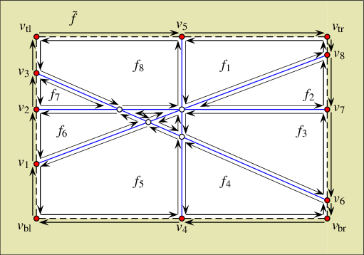
Figure 35.12 A DCEL representing an arrangement of four lines. Halfedges are drawn as thin arrows. The vertices \(v_1, \ldots, v_8\) lie at infinity, and are not associated with valid points. The halfedges that connect them are fictitious, and are not associated with concrete curves. The face denoted \(f_0\) (lightly shaded) is the fictitious "unbounded face" which lies outside the bounding rectangle (dashed) that bounds the actual arrangement. The four fictitious vertices \(v_{\rm bl}, v_{\rm tl}, v_{\rm br}\) and \(v_{\rm tr}\) represent the four corners of the imaginary bounding rectangle.
Instead of an explicit approach, we use an implicit bounding rectangle embedded in the DCEL structure. Figure 35.12 shows the arrangement of four lines that subdivide the plane into eight unbounded faces and two bounded ones. Notice that in this case portions of the the unbounded faces now have outer boundaries (those portions inside the bounding rectangle), and the halfedges along these outer CCBs are drawn as arrows. The bounding rectangle is drawn dashed. The vertices \(v_1,v_2,\ldots,v_8\), which lie on the bounding rectangle, represent the unbounded ends of the four lines that approach infinity. The halfedges connecting them, which overlap with the bounding rectangle, are not associated with geometric curves. Thus, we refer to them as fictitious. Note that the outer CCBs of the unbounded faces contain fictitious halfedges. The twins of these halfedges form together one connected component that corresponds to the entire imaginary rectangle. It forms a single hole in the face \(\tilde{f}\). We refer to \(\tilde{f}\) as fictitious, since it does not correspond to a real two-dimensional cell of the arrangement. Finally, there are four additional vertices denoted by \(v_{\rm bl}, v_{\rm tl}, v_{\rm br}\), and \(v_{\rm tr}\), which coincide with the bottom-left, top-left, bottom-right, and top-right corners of the bounding rectangle, respectively. They do not lie on any curve, and are referred to as fictitious as well. These four vertices identify each of the fictitious edges as lying on the top, the bottom, the left, and the right edge of the imaginary bounding rectangle. The four fictitious vertices exist even when the arrangement is empty: In this case they are connected by four pairs of fictitious halfedges that define a single unbounded face (which represents the entire \(\mathbb{R}^2\) plane) lying inside the imaginary bounding rectangle and a fictitious face lying outside.
In summary, there are four types of arrangement vertices, which differ from one another by their location with respect to the imaginary bounding rectangle as follows:
A vertex, associated with a point in \(\mathbb{R}^2\). Such a vertex always lies inside the bounding rectangle and has bounded coordinates..
A vertex that represents an unbounded end of an \(x\)-monotone curve that approaches \(x = -\infty\) or at \(x = \infty\). In case of a horizontal line or a curve with a horizontal asymptote, the \(y\)-coordinate of the curve end may be finite (see, for example, the vertices \(v_2\) and \(v_7\) in Figure 35.12), but in general the curve end also approaches \(y = \pm\infty\); see for instance the vertices \(v_1\), \(v_3\), \(v_6\) and \(v_8\) in Figure 35.12). For convenience, we always take a "tall" enough bounding rectangle and treat such vertices as lying on either the left or the right rectangle edges (that is, if a curve approaches \(x = -\infty\), its left end will be represented by a vertex on the left edge of the bounding rectangle, and if it approaches \(x = \infty\), its right end will be represented by a vertex on the right edge).
A vertex that represents the unbounded end of a vertical linear curve (line or ray) or of a curve with a vertical asymptote (finite \(x\)-coordinate and an unbounded \(y\)-coordinate). Such a vertex always lies on one of the horizontal edges of the bounding rectangle (either the bottom one if \(y = -\infty\), or the top one if \(y = \infty\)). The vertices \(v_4\) and \(v_5\) in Figure 35.12 are of this type.
The fictitious vertices that represent the four corners of the bounding rectangle.
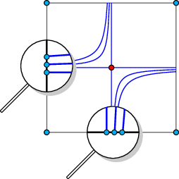
Figure 35.13 The portions of a horizontal line, a vertical line, and two rectangular hyperbolas with horizontal and vertical asymptotes confined to the imaginary bounding rectangle.
A vertex (at infinity) of Type 2 or Type 3 above always has three incident edges—one concrete edge that is associated with an unbounded portion of an \(x\)-monotone curve, and two fictitious edges connecting the vertex to its neighboring vertices at infinity or the corners of the bounding rectangle; see Figure 35.13. Fictitious vertices (of type 4 above) have exactly two incident fictitious edges. See Section The Geometry Traits for an explanation on how the traits-class interface helps impose the fact that a vertex at infinity is incident to a single non-fictitious edge.
The traits class that substitutes the Traits parameter of the Arrangement_2<Traits,Dcel> class template when the latter is instantiated specifies whether the arrangement instance supports unbounded curves through the definitions of some tags nested in the traits class; see Section The Basic Concept for details. Every arrangement that supports unbounded curves supports bounded curves as well, but not vice versa. Maintaining an arrangement that supports unbounded curves incurs an overhead due to the necessity to manage the imaginary bounding rectangle. If you know beforehand that all input curves that induce a particular arrangement are bounded, define your arrangement accordingly. That is, use a traits class that does not support unbounded curves.
The types Vertex, Halfedge, and Face nested in the Arrangement_2 class template support the methods described below in addition to the ones listed in Section Traversing the Arrangement. Let \(v\), \(e\), and \(f\) be handles to a vertex of type Vertex, a halfedge of type Halfedge, and a face of type Face, respectively.
The calls v->parameter_space_in_x() and v->parameter_space_in_y() determine the location of the geometric embedding of the vertex \(v\). The call v->parameter_space_in_x() returns CGAL::ARR_INTERIOR if the \(x\)-coordinate associated with \(v\) is finite, CGAL::ARR_LEFT_BOUNDARY if \(v\) represents the end of a curve the \(x\)-coordinate of which approaches \(-\infty\), and CGAL::ARR_RIGHT_BOUNDARY if \(v\) represents the end of a curve the \(x\)-coordinate of which approaches \(\infty\). Similarly, the call v->parameter_space_in_y() returns CGAL::ARR_INTERIOR if the \(y\)-coordinate associated with \(v\) is finite and CGAL::ARR_BOTTOM_BOUNDARY or CGAL::ARR_TOP_BOUNDARY if \(v\) represents the end of a curve the \(y\)-coordinate of which approaches \(-\infty\) or \(\infty\), respectively.
The nested Vertex type also provides the Boolean predicate is_at_open_boundary(). If the call v->is_at_open_boundary() predicates evaluates to false, you can access the point associated with \(v\). Otherwise, \(v\) is not associated with a Point_2 object, as it represents the unbounded end of a curve that approaches infinity.
The nested Halfedge type provides the Boolean predicate is_fictitious(). If the call e->is_fictitious() evaluates to false, you can access the \(x\)-monotone curve associated with \(e\). Otherwise, \(e\) is not associated with an X_monotone_curve_2 object.
The nested Face type provides the Boolean predicate is_fictitious(). The call f->is_fictitious() evaluates to true only when \(f\) lies outside the bounding rectangle. The method outer_ccb() (see Section Traversal Methods for an Arrangement Face must not be invoked for the fictitious face. Typically, the code is guarded against such malicious calls with adequate preconditions. However, these preconditions are suppressed when the code is compiled with maximum optimization. Note that a valid unbounded face (of an arrangement that supports unbounded curves) has a valid outer CCB, although the CCB comprises only fictitious halfedges if the arrangement is induced only by bounded curves.
Let \(p_l = (x_l,y_l)\) and \(p_r = (x_r,y_r)\) be the left and right endpoints of a bounded \(x\)-monotone curve \(c\), respectively. We say that a point \(p = (x_p,y_p)\) lies in the \(x\)-range of \(c\) if \(x_l \leq x_p \leq x_r\). Let \(p_l = (x_l,y_l)\) be the left endpoint of an \(x\)-monotone curve \(c\) unbounded from the right. A point \(p = (x_p,y_p)\) lies in the \(x\)-range of \(c\) if \(x_l \leq x_p\). Similarly, A point \(p = (x_p,y_p)\) lies in the \(x\)-range of an \(x\)-monotone curve unbounded from the left if \(x_p \leq x_r\). Naturally, every point \(p \in \mathbb{R}^2\) is in the \(x\)-range of an \(x\)-monotone curve unbounded from the left and from the right.
The function template is_in_x_range() listed below, and defined in the file is_in_x_range.h, checks whether a given point \(p\) is in the \(x\)-range of the curve associated with a given halfedge \(e\). The function template also exemplifies how some of the above functions can be used. The traits functor Compare_x_2 used in the code is described in Section The Basic Concept.
It is important to observe that the call arr.number_of_vertices() does not count the vertices at infinity in the arrangement arr. To find out this number you need to issue the call arr.number_of_vertices_at_infinity(). Similarly, arr.number_of_edges() does not count the fictitious edges (whose number is always arr.number_of_vertices_at_infinity() + 4) and arr.number_of_faces() does not count the fictitious faces. The vertex, halfedge, edge, and face iterators defined by the Arrangement_2 class template only go over true features of the arrangement; namely, vertices at infinity and fictitious halfedges and fictitious faces are skipped. On the other hand, the Ccb_halfedge_circulator of the outer boundary of an unbounded face or the Halfedge_around_vertex_circulator of a vertex at infinity do traverse fictitious halfedges. While an arrangement induced by bounded curves has a single unbounded face, an arrangement induced by unbounded curves may have several unbounded faces. The call arr.number_of_unbounded_faces() returns the number of unbounded arrangement faces (Thus, arr.number_of_faces() - arr.number_of_unbounded_faces() is the number of bounded faces). The calls arr.unbounded_faces_begin() and arr.unbounded_faces_end() return iterators of the type Arrangement_on_surface_2::Unbounded_face_iterator (or its non-mutable, const, counterpart type) that define the range of the arrangement unbounded faces. Naturally, the value-type of this iterator is Face.
There is no way to directly obtain the fictitious vertices that represent the four corners of the imaginary bounding rectangle. However, you can obtain the fictitious face through the call arr.fictitious_face(), and then iterate over the boundary of its single hole, which represents the imaginary bounding rectangle. Recall that an arrangement of bounded curves does not have a fictitious face. In this case the call above returns a null handle.
The example below exhibits the difference between an arrangement induced by bounded curves, which has a single unbounded face, and an arrangement induced by unbounded curves, which may have several unbounded faces. It also demonstrates the usage of the insertion function for pairwise interior-disjoint unbounded curves. In this case we use an instance of the traits class-template Arr_linear_traits_2<Kernel> to substitute the Traits parameter of the Arrangement_2<Traits,Dcel> class template when instantiated. This traits class-template is capable of representing line segments as well as unbounded linear curves, namely, lines and rays. Observe that objects of the X_monotone_curve_2 type nested in this traits class-template are constructible from objects of types Line_2, Ray_2, and Segment_2 also nested in the traits class-template. These three types and the Point_2 type are defined by the traits class-template Arr_linear_traits_2<Kernel> to be the corresponding types of the kernel used to instantiate the traits class-template; see Paragraph The Linear-Traits Class.
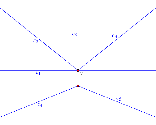
Figure 35.14 An arrangement of unbounded linear objects, as constructed in Arrangement_on_surface_2/unbounded_non_intersecting.cpp.
The first three curves, \(c_1\), \(c_2\), and \(c_3\), are inserted using the specialized insertion functions for \(x\)-monotone curves whose location in the arrangement is known. Notice that inserting an unbounded curve in the interior of an unbounded face, or from an existing vertex that represents an bounded end of the curve, may cause an unbounded face to split. (This is never the case when inserting a bounded curve—compare with Section Inserting Pairwise Disjoint x-Monotone Curves.) Three additional rays are then inserted incrementally using the insertion function for \(x\)-monotone curves, the interior of which is disjoint from all arrangement features; see the illustration in Figure 35.14). Finally, the program prints the size of the arrangement using the function template print_unbounded_arrangement_size() defined in the header file arr_print.h. (Its listing is omitted here.) The program also traverses the outer boundaries of its six unbounded faces and prints the curves along these boundaries. The header file arr_linear.h, which contains the definitions used by the example program, is listed immediately after the listing of the main function.
File Arrangement_on_surface_2/unbounded_non_intersecting.cpp
The type definitions used by the example below, as well as by other examples that use the Arr_linear_traits_2 class template, are listed next. These types are defined in the header file arr_linear.h.
All the free functions that operate on arrangements of bounded curves (see Section Free Functions) can also be applied to arrangements of unbounded curves. For example, consider a container of linear curves that has to be inserted into an arrangement object, the type of which is an instance of the Arrangement_2<Traits,Dcel> class template, where the Traits parameter is substituted by the traits class that handles linear curves; see Section The Linear-Traits Class. You can do it incrementally; namely, insert the curves one by one as follows:
Alternatively, the curves can be inserted aggregately using a single call as follows:
It is also possible to issue point-location queries and vertical ray-shooting queries (see also Section Issuing Queries on an Arrangement) on arrangements of lines, where the only restriction is that the query point has finite coordinates. Note that all the point-location strategies mentioned above, except the trapezoidal map strategy, are capable of handling arrangements of unbounded curves.
In the following example we show how an arrangement of unbounded lines is utilized to solve the following problem: Given a set of points, does the set contain at least three collinear points? In this example a set of input points is read from a file. The file points.dat is used by default. It contains definitions of \(100\) points randomly selected on the grid \([-10000,10000]\times[-10000,10000]\). We construct an arrangement of the dual lines, where the line \(p^{*}\) dual to the point \(p = (x_p, y_p)\) is given by the equation \(y =
x_p*x - y_p\), and check whether three (or more) of the dual lines intersect at a common point, by searching for a (dual) vertex, whose degree is greater than \(4\). If such a vertex exists, then there are at least three dual lines that intersect at a common point, which implies that there are at least three collinear points.
File Arrangement_on_surface_2/dual_lines.cpp
Note that there are no three collinear points among the points defined in the input file points.dat. In the second part of the example the existence of a collinear triple is forced and verified as follows. A line dual to the midpoint of two randomly selected points is introduced, and inserted into the arrangement. This operation is followed by a test that verifies that a vertex of degree greater than \(4\) exists.
We are given a surface \(S\) in \(\mathbb{R}^3\) and a set \(\mathcal{C}\) of curves embedded in this surface. The curves subdivide \(S\) into cells of dimension 0 (vertices), 1 (edges), and 2 (faces). This subdivision is the arrangement \(\mathcal{A}(\mathcal{C})\) induced by \(\mathcal{C}\) on \(S\). Arrangements embedded in curved surfaces in \(\mathbb{R}^3\) are generalizations of arrangements embedded in the plane. In this section we explain how to construct, maintain, and manipulate two-dimensional arrangements embedded in orientable parametric surfaces in three dimensions, such as planes, cylinders, spheres, and tori, and surfaces homeomorphic to them; see Figure 35.15. Such arrangements have many theoretical and practical applications; see, e.g., [1], [3], [4], [6], and [8].

| 
| 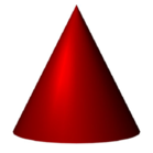
| 
| 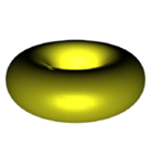
| 
|
| (a) Sphere | (b) Cylinder | (c) Cone | (d) Ellipsoid | (e) Torus | (f) Paraboloid |
Figure 35.15 Various two-dimensional parametric surfaces, arrangements on which are supported by the framework.
We use \(\overline{\mathbb{R}}\) to denote the compactified real line \(\mathbb{R} \cup \{-\infty,+\infty\}\). The mapping \(x \mapsto x/(1 - x^2)\) is a homeomorphism between \((-1,+1)\) and \(\mathbb{R}\) and between \([-1,+1]\) and \(\overline{\mathbb{R}}\). So you may also think of finite intervals instead of the (compactified) real line in what follows.
A parametric surface \(S\) is given by a continuous function \(\phi_S: \Phi \rightarrow \mathbb{R}^3\), where the domain \(\Phi = X \times Y\) is a rectangular two-dimensional parameter space and \(S = \phi_S(\Phi)\). The sets \(X\) and \(Y\) are open, half-open, or closed intervals with endpoints in \(\overline{\mathbb{R}}\). We use \(x_{\rm min}\), \(x_{\rm max}\), \(y_{\rm min}\), and \(y_{\rm max}\) to denote the endpoints of \(X\) and \(Y\), respectively.
The left side of the boundary of \(\Phi\) consists of the points \((x_{\rm min},y)\) with \(y \in {\rm closure}(Y)\). It is open, if \(x_{\rm min} \not\in X\) or \(y\not\in Y\), and closed, otherwise. The right side is defined analogously. The bottom side consists of the points \((x, y_{\rm min})\) with \(x \notin (x_{\rm min},x_{\rm max})\); the top side is defined analogously. The bottom or top sides can also be open. Note that the "corners" of the parameter space belong to the vertical sides; this asymmetry corresponds to the fact that we sweep \(x\)-monotone curves, and not \(y\)-monotone curves. The four sides together form the boundary \(\partial \Phi\).
A point \(p \in S\) is regular if it has only one pre-image under \(\Phi\). All pre-images of a non-regular point lie in the boundary of \(\Phi\). In particular, \(\phi_S\) is bijective on \((x_{\rm min},x_{\rm max})\times(y_{\rm min},y_{\rm max})\). More precisely, a non-regular point has either exactly two pre-images that lie on opposite sides of the domain, or all points of exactly one side of the domain.
A side of the domain is contracted if \(\phi_S\) is constant on it. The image of the side is called a contraction point.
The bottom and top sides of the domain (similarly for the left and right sides) are identified if \(\phi_S(x,y_{\rm min}) = \phi_S(x, y_{\rm max})\) for all \(x \in X \). The curve \(x \mapsto \phi_S(x,y_{\rm min})\) is called an identification curve.
Rectangles, strips, quadrants, half-planes, and planes can be modeled with \(\phi_S \) being the identity mapping. For example, \(\Phi_S(x, y) = (x, y, 0)\) with \(X = Y =(-\infty, +\infty)\) parameterizes a plane. Surfaces such as paraboloids can be modeled through continuous and bijective parameterizations, for example, \(\phi_S(x,y) = (x,y,x^2 + y^2)\), where \(U = V =(-\infty, +\infty)\), defines a paraboloid of revolution. Cylinders, tori, spheres, and surfaces homeomorphic to them, require more general parameterizations. For example, the unit sphere is commonly parameterized as \(\phi_S(x, y) = (\cos x \cos y, \sin x \cos y, \sin y)\), where \(\Phi = [-\pi, \pi] \times [-\frac{\pi}{2}, \frac{\pi}{2}]\). With respect to this parameterization, the north and the south pole and all points on the opposite Prime (Greenwich) Meridian are non-regular. The north pole \((0,0,1)\) has infinitely many pre-images \((x, \pi/2)\) with \(-\pi < x < \pi\) and so does the south pole \((0,0,-1)\). The points on the opposite Prime Meridian have two pre-images each, namely \((-\pi,y)\) and \((\pi,y)\) with \(-\pi/2 \leq y \leq \pi/2\). We say that the top and bottom side of the domain are contracted and the left and right sides are identified. These are exactly the kinds of non-injectivity that we allow.
We give more examples. A triangle with corners \((a_1, b_1), (a_2, b_2)\), and \((a_3, b_3)\) can be parameterized via \(\Phi = [0,1] \times [0,1]\) with \(\phi_S(x,y) = (a_1 + x(a_2 - a_1) + xy(a_3-a_2), b_1 + x(b_2 - b_1) + xy(b_3-b_2), 0)\). The left side of the rectangular domain contracts to a point. An open or closed cylinder is modeled by identifying the vertical sides and having \(Y\) open or closed, respectively. A torus is modeled by identifying the vertical sides and the horizontal sides. A paraboloid or half-cone may be modeled by identifying the vertical sides and contracting one of the horizontal sides to a point. More elegantly, they are modeled by a bijective parameterization as given above. A sphere is modeled by identifying the vertical sides and contracting both horizontal sides. A croissant, a torus with one pinch point, is modeled by identifying the vertical and identifying the horizontal sides and, in addition, contracting one of the pairs. However, the croissant is excluded by our definitions. All surfaces supported by our framework are locally homeomorphic to a disk, and hence an DCEL data-structure suffices for representing arrangements on these surfaces. The croissant is, at the pinch point, not locally homeomorphic to a disk, and hence a more general cell-tuple data structure than an DCEL would be needed.
A curve \(\gamma\) is a continuous function \(\gamma: I \rightarrow \Phi\), where \(I\) is an open, half-open, or closed interval with endpoints 0 and 1, and \(\gamma\) is injective except at a finite number of points. If \(0 \not\in I\), the limit \(\lim_{t \rightarrow 0+} \gamma(t)\) exists (in the closure of \(\Phi\)) and lies in an open side of the boundary. Similarly, if \(1 \not\in I\), then \(\lim_{t \rightarrow 1-} \gamma(t)\) exists and lies in an open side of the boundary. A curve \(c\) in \(S\) is the image of a curve \(\gamma\) in the domain.
A curve is closed in the domain if \(\gamma(0) = \gamma(1)\); in particular, \(0 \in I\) and \(1 \in I\). A curve is closed in the surface \(S\) (or simply closed) if \(\phi_S(\gamma(0)) = \phi_S(\gamma(1))\). A curve \(\gamma\) has two ends, the 0-end \(\langle \gamma,0 \rangle\) and the 1-end \(\langle \gamma,1 \rangle\). If \(d \in I\), the \(d\)-end has a geometric interpretation. It is a point in \(\Phi\). If \(d \not\in I\), the \(d\)-end has no geometric interpretation. You may think of it as a point on an open side of the domain or an initial or terminal segment of \(\gamma\). If \(d \not\in I\), we say that the \(d\)-end of the curve is open. The equator curve on the sphere in standard parameterization is given by \(\gamma(t) = (\pi(2t - 1),0)\) for \(t \in [0,1]\). The \(0\)-end of \(\gamma\) is the point \((-\pi,0)\) in \(\Phi\) and a point on the equator of the sphere. It is closed on the sphere, but not closed in \(\Phi\). The diagonal \((u,u)\) in the plane is, for example, given by \(\gamma(t) = (x(t),y(t))\) and \(x(t) = y(t) = (t - 1/2)/(t(1-t))\). Both ends of this curve are open. The \(d\)-end of a curve \(\gamma\) is incident to the left side if either \(d \in I\) and \(\gamma(d)\) lies on the left side or \(d \not\in I\) and \(\lim_{t \rightarrow d} \gamma(t)\) lies on the left side, which is then an open side. Similarly for the other sides.
A strongly \(x\)-monotone curve is the image of a curve \(\gamma\), such that if \(t_1 < t_2\) for \(t_1, t_2 \in I\), then \(x(t_1) < x(t_2)\). A vertical curve is the image of a curve \(\gamma\), such that \(x(t) = C\) for all \(t \in I\) and some \(C \in X\) and \(y(t_1) < y(t_2)\) for \(t_1 < t_2\). For instance, every Meridian curve of a sphere parameterized as above is vertical. An \(x\)-monotone curve is either vertical or strongly \(x\)-monotone.
The class template Arrangement_on_surface_2<GeomTraits, TopolTraits> can be used to represent a 2D arrangement embedded in a 3D surface. The template is parameterized by template parameters geometry traits and topology traits. The topology-traits type deals with the topology of the parametric surface; see Section The Topology Traits. As explained in the previous section, a parametric surface \(S = \phi_S(\Phi)\) is given by a continuous function \(\phi_S: \Phi \rightarrow \mathbb{R}^3\), where the domain \(\Phi = X \times Y\) is a rectangular two-dimensional parameter space. \(X\) and \(Y\) are open, half-open, or closed intervals with endpoints in \(\overline{\mathbb{R}}\).
The geometry-traits type introduces the type names of the basic geometric objects (i.e., point, curve, and \(x\)-monotone curve) and the set of operations on objects of these types required to construct and maintain the arrangement and to operate on it. The traits-concept hierarchy described in Section The Geometry Traits accurately defines the requirements imposed on a model of a geometry traits class. Recall that requirements apply to the parameter space \(\Phi = X \times Y\); thus, they are defined in terms of \(x\) and \(y\) coordinates. Most requirements apply to all type of arrangements regardless of the embedding surface. However, several refined concepts apply only to arrangements on surfaces that are not in the plane, that is, modeled with \(\phi_S\) not being the identity mapping. They differ according to the type of the side boundaries of the parameter space being open, closed, contracted, or identified.
At this point only one type of arrangements on non planar surfaces is supported, namely, arrangements embedded in the sphere and induced by arcs of great circles, also known as geodesic arcs. Figure 35.16 shows various Voronoi diagrams the bisectors of which are geodesic arcs. They are represented as arrangements induced by geodesic arcs embedded in the sphere.
| 
| 
| 
|
| (a) | (b) | (c) | (d) |
Figure 35.16 Voronoi diagrams on the sphere. All diagram edges are geodesic arcs. Sites are drawn in red and Voronoi edges are drawn in blue. (a) The Voronoi diagram of 32 random points. (b) A highly degenerate case of Voronoi diagram of 30 point sites on the sphere. (c) The power diagram of 10 random circles. (d) A degenerate power diagram of 14 sites on the sphere.
The types Vertex, Halfedge, and Face nested in the Arrangement_on_surface_2 class template support the methods listed in Section Traversing the Arrangement and in Section Basic Manipulation and Traversal Methods. Additional methods supported by these types are described next. Let \(v\), \(e\), and \(f\) be handles to a vertex of type Vertex, a halfedge of type Halfedge, and a face of type Face, respectively.
The calls v->parameter_space_in_x() and v->parameter_space_in_y() determine the location of the geometric embedding of the vertex \(v\). The call v->parameter_space_in_x() returns ARR_INTERIOR if the geometric embedding of \(v\) is a point \(p\) the pre-image of which does not lie on the left nor on the right sides of the boundary of the parameter space. If the left and right sides are not identified, then ARR_LEFT_BOUNDARY or ARR_RIGHT_BOUNDARY are returned if the pre-image of \(p\) lies on the left or the right side, respectively. If the left and right sides are identified, the return value is unspecified and can be either ARR_LEFT_BOUNDARY or ARR_RIGHT_BOUNDARY. Similarly, the call v->parameter_space_in_y() returns ARR_INTERIOR if the geometric embedding of \(v\) is a point \(q\), the pre-image of which does not lie on the bottom nor on the top sides of the boundary of the parameter space. If the bottom and top sides are not identified, then ARR_BOTTOM_BOUNDARY or ARR_TOP_BOUNDARY are returned if the pre-image of \(q\) lies on the bottom or the top side, respectively. If the bottom and top sides are identified, the return value is unspecified.
If you want to determine whether the pre-image of a point \(p\) lies on identified sides, you need to employ one of the two traits functors Is_on_x_identification_2 or Is_on_y_identification_2; see Section Supporting Unbounded Curves or Curved Surfaces. If the pre-image of an \(x\)-monotone curve \(c\) does not entirely lie on identified sides, you can determine the location of the pre-image of an endpoint of \(c\) employing either the Parameter_space_in_x_2 functor or the Parameter_space_in_y_2 functors; see Section Supporting Unbounded Curves or Curved Surfaces. The operations in both functors accept an enumeration that indicates the curve end, that is, CGAL::ARR_MIN_END or CGAL::ARR_MAX_END, in addition to the curve itself.
A face in a planar arrangement has at most one outer CCB. However, an arrangement embedded on a surface may present additional scenarios. For example, a face of an arrangement embedded on a torus may have two outer CCBs, and a face of an arrangement embedded on a sphere might be consider a hole inside the surrounding face or vice versa. To this end, outer CCBs and inner CCBs of faces of arrangements embedded on surfaces are symmetrically treated (while maintaining the invariant that a face always lies to the left of every halfedge of every CCB of the face regardless of whether the CCB is inner or outer). The classification of a CCB as inner or outer becomes an implementation detail. The calls f->outer_ccbs_begin() and f->outer_ccbs_end() return iterators of type Outer_ccb_iterator that define a range of outer CCBs inside the face \(f\). Similarly, the methods f->inner_ccbs_begin() and f->inner_ccbs_end() return iterators of type Inner_ccb_iterator that define a range of inner CCBs inside the face \(f\). (The latter pair of member functions and the iterator type are equivalent to the methods holes_begin(), holes_end(), and Hole_iterator; see Section Traversal Methods for an Arrangement Face.) The calls f->number_of_outer_ccbs() and f->number_of_inner_ccbs() return the number of outer CCBs and the number of inner CCBs in \(f\), respectively.
The function template is_in_x_range() listed below, and defined in the file spherical_is_in_x_range.h checks whether a given point \(p\), in the interior of the parameter space, is in the \(x\)-range of an \(x\)-monotone curve \(c\) that represents a great-circle arc. It assumes that the left and right sides of the parameter space are identified and the bottom and top sides are contracted, which is the settings used by the traits class template Arr_geodesic_arc_on_sphere_traits_2<Kernel,X,Y>; see Section Arcs of Great Circles Embedded in the Sphere. The traits functors Construct_min_vertex_2, Construct_min_vertex_2, and Compare_x_2 used in the code are described is Section The Basic Concept. The traits functors Parameter_space_in_x_2, Parameter_space_in_y_2, Is_on_y_identification_2, and Compare_x_on_boundary_2, are described is Section Supporting Unbounded Curves or Curved Surfaces.
A geometry traits class encapsulates the definitions of the geometric entities and the implementation of the geometric predicates and constructions that handle these geometric entities, used by the Arrangement_on_surface_2 class template and by the peripheral modules. The identified minimal requirements imposed by the various algorithms that apply to arrangements are organized in a hierarchy of refined geometry-traits concepts. The requirements listed by each concept include only the utterly essential types and operations needed to implement specific algorithms. This modular structuring yields controllable parts that can be produced, maintained, and utilized with less effort. For each operation, all the preconditions that its operands must satisfy are specified as well, as these may simplify the implementation of models of these concepts even further. Each traits class models one or more concepts. This section contains a detailed description of the concepts in the refinement hierarchy and the various traits classes that model these concepts.
All the algebra required for constructing and manipulating arrangements is concentrated in the traits classes. The knowledge required to devise a good traits class is very different from the knowledge required for the development of the rest of the package or for using the package. It has less to do with computational geometry and it involves mainly algebra and numerical computation. This way, traits classes for new types of curves can be developed with little knowledge of algorithms and data structures in computational geometry. In this section we discuss how to use existing traits classes, but we also explain the concepts these traits classes model—a starting point for every novice developer of such classes.
This section is divided into three parts. The first part describes the refinement hierarchy of the arrangement geometry-traits concepts. The second part reviews various models of these concepts. These traits classes handle different curve families, such as line segments, polylines, conic arcs, Bézier curves, algebraic curves, and geodesic arcs on the sphere. The last part introduces decorators for geometric traits classes. A decorator of a traits class attaches auxiliary data to the geometric objects handled by the original traits class, thereby extending it.
A hierarchy of related concepts can be viewed as a directed acyclic graph, where a node of the graph represents a concept and an arc represents a refinement relation. An arc directed from concept A to concept B indicates that concept B refines concept A. A rather large directed acyclic graph is required to capture the entire hierarchy of the geometry traits-class concepts. In the following sections we review individual clusters of the graph and describe the relations between them. Figure 35.17 depicts the central cluster.

Figure 35.17 The hierarchy of the main geometry traits concepts.
A model of the basic concept ArrangementBasicTraits_2 needs to define the types Point_2 and X_monotone_curve_2, where objects of the former type are the geometric mapping of arrangement vertices, and objects of the latter type are the geometric mapping of edges. In addition, it has to support the set of predicates listed below. This basic set of predicates is sufficient for constructing arrangements of bounded \(x\)-monotone curves that are pairwise disjoint in their interiors and points that do not lie in the interiors of the curves. The basic set of predicates is also sufficient for answering vertical ray-shooting queries and point-location queries with a small exception: Locating a point using the landmark strategy requires a traits class that models the concept ArrangementLandmarkTraits_2; see Section The Landmark Concept.
Compare_x_2: Compares the \(x\)-coordinates of two points.
Compare_xy_2: Compares two points lexicographically, first by their \(x\)-coordinates, and if they are equal, by their \(y\)-coordinates.
Equal_2: There are two overloaded Boolean operators that test equality. One returns true iff two given points represent the same geometric point in the two-dimensional surface, and the second returns true iff the graphs of two given \(x\)-monotone curves are the same.The predicate that tests equality between graphs of two \(x\)-monotone curves is used only for testing as part of the test suite.
Construct_min_vertex_2: Returns the lexicographically smallest (or left) endpoint of an \(x\)-monotone curve.
Construct_max_vertex_2: Returns the lexicographically largest (or right) endpoint of an \(x\)-monotone curve.
Is_vertical_2: Determines whether an \(x\)-monotone curve is vertical.
Compare_y_at_x_2: Given an \(x\)-monotone curve \(c\) and a point \(p\) that lies in the \(x\)-range of \(c\), determines whether \(p\) is below, above or lies on \(c\).
Compare_y_at_x_right_2: Every model of the concept ArrangementBasicTraits_2 needs to define a nested type named Has_left_category. It determines whether the traits class supports the following predicate:
Compare_y_at_x_left_2: Given two \(x\)-monotone curves \(c_1\) and \(c_2\) that share a common maximal (right) endpoint \(p\), determines whether \(c_1\) is above or under \(c_2\) immediately to the left of \(p\), or whether the two curves overlap there.
If the ArrangementBasicTraits_2::Has_left_category type nested in a model of the basic concept is defined as Tag_trueIn principle, the category type may only be convertible to the tag type, but in practice the category is typically explicitly defined as the tag. the model must support the predicate. If the type is defined as Tag_false, we resort to an internal version, which is based just on the reduced set of provided operations. The internal version might be less efficient, but it exempts the traits developer from the providing an (efficient) implementation of this predicate—a task that turns out to be nontrivial in some cases.
The basic set of predicates is sufficient for constructing arrangements of \(x\)-monotone curves that do not reach or approach the boundary of the parameter space. The nature of the input curves, whether they are expected to reach or approach the left, right, bottom, or top side of the boundary of the parameter space, must be conveyed by the traits class. This is done through the definition of four additional nested types, namely
Each of those types must be convertible to the type Arr_oblivious_side_tag for the class to be a model of the concept ArrangementBasicTraits_2.
Constructing an arrangement induced by \(x\)-monotone curves that may intersect in their interior requires operations that are not part of the ArrangementBasicTraits_2 concept. The additional operations are listed by the concept ArrangementXMonotoneTraits_2, which refines the basic arrangement geometry-traits concept described above. While models of the ArrangementXMonotoneTraits_2 concept still handle only \(x\)-monotone curves, the curves are not restricted to be disjoint in their interiors. Such a model must be capable of computing points of intersection between \(x\)-monotone curves, splitting curves at these intersection points to obtain pairs of interior-disjoint subcurves, and optionally merging pairs of subcurves. A point of intersection between two curves is also represented by the Point_2 type. A model of the refined concept must define an additional type called Multiplicity. An object of this type indicates the multiplicity of the intersection point of two curves, also referred to as the intersection number.See, e.g., https://en.wikipedia.org/wiki/Intersection_number for more information about intersection numbers. Loosely speaking, if two curves intersect at a point \(p\) but have different tangents (first derivatives) at \(p\), The point \(p\) is of multiplicity 1. If the curve tangents are equal but their curvatures (second derivatives) are not, \(p\) is of multiplicity 2, and so on. The multiplicity of points of intersection between line segments is always 1, and the multiplicity of a point of intersection between two polylines is 1 if the intersection point is interior to the corresponding two line segments of the polylines, and undefined (coded as 0) otherwise. A model of the refined concept thus has to support the following additional operations:
Split_2: Splits an \(x\)-monotone curve \(c\) into two subcurves at a given point \(p\) that lies in the interior of \(c\).
Are_mergeable_2: Determines whether two \( x\)-monotone curves \(c_1\) and \(c_2\) that share a common endpoint can be merged into a single continuous \(x\)-monotone curve representable by the traits class.On the face of it this seems a difficult predicate to implement. In practice we use very simple tests to decide whether two curves are mergeable: We check whether their underlying curves are identical and whether they do not bend to form a non- \(x\)-monotone curve.
Merge_2: Merges two mergeable \(x\)-monotone curves into a single curve.
Intersect_2: Computes all intersection points and overlapping sections of two given \(x\)-monotone curves. If possible, computes also the multiplicity of each intersection point. Providing the multiplicity of an intersection point is not required, but it can expedite the arrangement construction. Typically, the multiplicity is a byproduct of the intersection computation. However, if it is not available, undefined multiplicity (coded as 0) is assumed. Having the multiplicity of intersection points while constructing arrangements enables the exploitation of the geometric knowledge intersection points may have.
Using a model of the ArrangementXMonotoneTraits_2 it is possible to construct arrangements of sets of \(x\)-monotone curves (and points) that may intersect one another. The two operations listed above, regarding the merging of curves, are optional, and should be provided only if the type Has_merge_category nested in a model of the ArrangementXMonotoneTraits_2 concept is defined as Tag_true. Otherwise, it is not possible to merge \(x\)-monotone curve and redundant vertices may be left in the arrangement due to the removal of edges.
The concept ArrangementTraits_2 refines the ArrangementXMonotoneTraits_2 concept. A model of the refined concept must define an additional type that is used to represent general, not necessarily \(x\)-monotone and not necessarily continuous, curves, named Curve_2. It also has to support the subdivision of a curve of that type into a set of continuous \(x\)-monotone curves and isolated points. For example, the curve \(c:\ (x^2 + y^2)(x^2 + y^2 - 1) = 0\) comprises the unit circle (the locus of all points for which \(x^2 + y^2 = 1\)) and the origin (the singular point \((0,0)\)). \(c\) should therefore be subdivided into two circular arcs, the upper part and the lower part of the unit circle, and a single isolated point. In particular a model of the refined concept has to support the following additional operation:
Make_x_monotone_2: Divides a given general curve of type Curve_2 into continuous weakly \(x\)-monotone curves and isolated points.
Note that a model of the refined concept ArrangementTraits_2 is required only when using the free insert() function templates (see Section Free Functions) that accept an object of type Curve_2 or a range of objects of that type. In all other cases it is sufficient to use a model of the ArrangementXMonotoneTraits_2 concept.

Figure 35.18 The traits-concept hierarchy for arrangements associated with the landmark point-location strategy.
The type of an arrangement associated with the landmark point-location strategy (see Section Point-Location Queries) must be an instance of the Arrangement_on_surface_2<GeomTraits, TopolTraits> class template, where the GeomTraits parameter is substituted by a model of the concept ArrangementLandmarkTraits_2. (Naturally, it can also model either the ArrangementXMonotoneTraits_2 concept or the ArrangementTraits_2 concept.) The ArrangementLandmarkTraits_2 concept refines the two concepts ArrangementApproximateTraits_2 and ArrangementConstructXMonotoneCurveTraits_2. Each of these two concepts, in turn, refines the concept ArrangementBasicTraits_2.
A model of the ArrangementApproximateTraits_2 concept must define a fixed precision number type (typically the double-precision floating-point double) and support the operation below (in addition to fulfilling the requirements listed by the ArrangementBasicTraits_2 concept).
Approximate_2: Given a point p, approximate the \(x\) and \(y\)-coordinates of p using a not necessarily multi-precision number type. We use this operation for approximate computations—there are certain operations performed during the search for the location of the point that need not be exact, and that can be performed faster when carried out, for example, using a fixed-precision number type.
A model of the ArrangementConstructXMonotoneCurveTraits_2 concept must support the operation below (in addition to fulfilling the requirements listed by the ArrangementBasicTraits_2 concept).
Construct_x_monotone_curve_2: Given two points \(p_1\) and \(p_2\), construct an \(x\)-monotone curve connecting \(p_1\) and \(p_2\).
Most traits classes model the ArrangementTraits_2 concept, and some also model the ArrangementLandmarkTraits_2 concept.
The concept ArrangementConstructCurveTraits_2 refines the concept ArrangementTraits_2. A model of the ArrangementConstructCurveTraits_2 concept must support the operation below (in addition to fulfilling the requirements listed by the ArrangementTraits_2 concept).
Construct_curve_2: The Arr_polyline_traits_2<SubcurveTraits_2> class template handles polylines; see Section ~The Polyline Traits Class. The type that substitutes the template parameter SubcurveTraits_2 when Arr_polyline_traits_2<SubcurveTraits_2> is instantiated must be a geometry-traits class that models the concept ArrangementConstructCurveTraits_2 to enable the construction of polylines from a sequence of two or more points.
We descend to the bottom level of the hierarchy. The refinements described in this section provide the requirements imposed on traits classes used with arrangements induced by curves with boundary conditions. In particular, these requirements list additional operations that handle curves that either reach specific sides of the parameter-space boundary (the pre-images of their endpoints lie on boundary sides) or approach them (the pre-images of their endpoints approach boundary sides). These boundary conditions typically occur with unbounded curves or with arrangements embedded in curved surfaces. The category types Left_side_category, Right_side_category, Bottom_side_category, and Top_side_category, nested in every geometry traits class indicate whether the corresponding boundary side (i.e., left, right, bottom, and top) is open, closed, contracted, or identified, and whether this information is relevant at all. When all curves inserted into the arrangement are expected to neither approach nor reach that particular boundary side, the information is irrelevant. (Note that we explicitly distinguish closed-only, contracted, and identified sides, although the latter two are closed in the parameter space as well.) Each one of the categories above must be convertible to one of the tag types listed below according to the boundary condition that should be handled.
For each of the four sides of the parameter space there are four available concepts, models of which can be used to handle open, closed, contracted, and identified sides, respectively. (When curves are expected to neither reach nor approach a particular side, special handling is not required; thus, there is no need for a corresponding concept.) For example, it is required that the category type Bottom_side_category, nested in models of the concept ArrangementOpenBottomTraits_2, is convertible to the tag type Arr_open_side_tag. This makes for a total of 16 abstract concepts (combine one of left, right, bottom, and top with one of open, closed, contracted, identified). Any one of these individual abstract concept is useless on its own; only concepts that refine a combination of 0, 1, 2, 3, or 4 abstract concepts (which capture the conditions that occur in the four sides simultaneously) are purposeful. Theoretically, there are \(\sum_{i=0}^4\binom{i}{4} \cdot 4^i = 5^4 = 625\) such concepts. However, only a subset of them is meaningful. If a side is identified, the opposite side must also be identified. In addition, a contracted side must be adjacent to two identified sides. While this narrows down the number of tangible concepts, the total number is still high; in practice we have used only two so far (not counting the "plain" concept, models of which do not handle boundary conditions at all), namely, ArrangementOpenBoundaryTraits_2 and ArrangementSphericalBoundaryTraits_2; see below for more details. Many of the traits class-templates provided by the 2D Arrangements package do not handle boundary conditions at all. Some of them, such as the Arr_segment_traits_2 traits (see Section Traits Classes for Line Segments and Linear Objects) only handle bounded curves. Thus, the four category types nested in these models are defined to be Arr_oblivious_side_tag.

Figure 35.19 Bottom portion of the refinement hierarchy of the geometry-traits concepts for curves embedded in an open surface, for instance, the entire plane.
Several predicates are required to handle \(x\)-monotone curves that approach the boundary of the parameter space. These predicates are sufficient to handle not only curves embedded in an unbounded parameter space, but also curves embedded in a bounded parameter space with open boundaries. The arrangement type instantiated with a traits class that models the combined concept ArrangementOpenBoundaryTraits_2 shown in Figure 35.19 can handle curves that are open in any direction. Recall that an arrangement that supports unbounded \(x\)-monotone curves maintains an implicit bounding rectangle in the DCEL structure; see Section Arrangements of Unbounded Curves. If some curves inserted into an arrangement object are expected to be unbounded; namely, there exists \(d \in \{0,1\}\) such that \(\lim_{t \rightarrow d}x(t) = \pm\infty\) or \(\lim_{t
\rightarrow d}y(t) = \pm\infty\) holds for at least one input curve \(c(t) = (x(t),y(t))\), the arrangement template must be instantiated with a model of the ArrangementOpenBoundaryTraits_2 concept.A curve that reaches the boundary of the parameter space in this case is open and unbounded.

Figure 35.20 Bottom portion of the refinement hierarchy of the geometry-traits concepts for curves embedded in a sphere-like parameterized surface
A suitable geometry-traits component for arrangements embedded in surfaces homeomorphic to a sphere is a model of the combined concept ArrangementSphericalBoundaryTraits_2 shown in Figure 35.20. Here the two vertical sides of the parameter space are identified and the two horizontal sides are contracted.

Figure 35.21 Top portion of the refinement hierarchy of the geometry-traits concepts for curves that either reach the left side of the boundary of the parameter space or approach it. A similar hierarchy also exists for the right, bottom, and top sides.
The shared requirements for the four options of a side are collected in abstract layers called ArrangementLeftSideTraits_2, ArrangementRightSideTraits_2, ArrangementBottomSideTraits_2, and ArrangementTopSideTraits_2; see, e.g., Figure 35.21.

Figure 35.22 Top portion of the refinement hierarchy of the geometry-traits concepts for curves that either reach the vertical sides of the boundary of the parameter space or approach it, and similarly for curves that either reach or approach horizontal sides.
The shared requirements for the options of opposite sides are collected in two additional abstract layers called ArrangementVerticalSideTraits_2 and ArrangementHorizontalSideTraits_2; see Figure 35.22.

Figure 35.23 Top portion of the refinement hierarchy of the geometry-traits concepts for curves that reach the identified vertical sides of the parameter space and for curves that reach the identified horizontal sides of the parameter space.
Individual concepts for curves that reach the identified left side of the parameter space and for curves that reach the identified right side of the parameter space do not exist, because if one side is identified the opposite side must be identified as well. Similarly, individual concepts for curves that reach the identified bottom side of the parameter space and for curves that reach the identified top side of the parameter space do not exist either. Instead, the shared requirements for opposite identified sides are collected in two additional abstract concepts called ArrangementIdentifiedVerticalTraits_2 and ArrangementIdentifiedHorizontalTraits_2; see Figure 35.23. The former lists requirements for operations that handle curves that reach identified vertical sides of the parameter space, and the latter lists requirements for operations that handle curves that reach identified horizontal sides of the parameter space.
In the following we list the specific requirements of all the aforementioned concepts.
The abstract concept ArrangementVerticalSideTraits_2 requires the following predicate:
Parameter_space_in_x_2: This three-valued predicate is overloaded with two versions as follows:
(i) Given a curve \(c = (x(t), y(t))\) and an enumerator that specifies either the minimum end or the maximum end of the curve, and thus maps to a parameter value \(d \in \{0,1\}\), determine the location of the \(d\)-end of \(c\) along the \(x\)-dimension. Formally, if \(c\) is open at its \(d\)-end, determine whether \(\lim_{t \rightarrow d} x(t)\) evaluates to \(x_{\rm min}\), \(x_{\rm max}\), or a value in between. If \(c\) is not open at its \(d\)-end, determine whether \(x(d)\) is equal to \(x_{\rm min}\), \(x_{\rm max}\), or a value in between. Return CGAL::ARR_LEFT_BOUNDARY, CGAL::ARR_RIGHT_BOUNDARY, or CGAL::ARR_INTERIOR, accordingly. If \(c\) is vertical and lies on a vertical boundary; that is, either \(\forall p=(x_p, y_p) \in c\) we have \(x_p = x_{\rm min}\) or \(\forall p=(x_p, y_p) \in c\) we have \(x_p = x_{\rm max}\), then the boundary side containing \(c\) cannot be open.
(ii) Given a point \(p=(x_p, y_p)\), determine the location of the point with respect to the \(x\)-axis. Formally, determine whether \(x_p\) is equal to \(x_{\rm min}\), \(x_{\rm max}\), or a value in between. Return CGAL::ARR_LEFT_BOUNDARY, CGAL::ARR_RIGHT_BOUNDARY, or CGAL::ARR_INTERIOR, accordingly. If \(p\) is on a vertical boundary; that is, \(x_p \in \{x_{\rm
min},x_{\rm max}\}\), then the boundary side containing \(p\) cannot be open and must not be identified. In other words, this overloaded version is required only for the concepts ArrangementClosedLeftTraits_2, ArrangementClosedRightTraits_2, ArrangementContractedLeftTraits_2 and ArrangementContractedRightTraits_2.
The abstract concept ArrangementHorizontalSideTraits_2 requires the following predicate:
Parameter_space_in_y_2: This three-valued predicate is overloaded with two versions as follows:
(i) Given a curve \(c = (x(t), y(t))\) and an enumerator that specifies either the minimum end or the maximum end of the curve, and thus maps to a parameter value \(d \in \{0,1\}\), determine the location of the \(d\)-end of \(c\) along the \(y\)-dimension. Formally, if \(c\) is open at its \(d\)-end, determine whether \(\lim_{t \rightarrow d} y(t)\) evaluates to \(y_{\rm min}\), \(y_{\rm max}\), or a value in between. If \(c\) is not open at its \(d\)-end, determine whether \(y(d)\) is equal to \(y_{\rm min}\), \(y_{\rm max}\), or a value in between. Return CGAL::ARR_BOTTOM_BOUNDARY, CGAL::ARR_TOP_BOUNDARY, or CGAL::ARR_INTERIOR, accordingly. If \(c\) is horizontal and lies on a horizontal boundary; that is, either \(\forall p=(x_p, y_p)
\in c, y_p = y_{\rm min}\) or \(\forall p=(x_p, y_p) \in c, y_p =
y_{\rm max}\), then the boundary side containing \(c\) cannot be open and must not be identified.
(ii) Given a point \(p=(x_p, y_p)\), determine the location of the point along the \(y\)-dimension. Formally, determine whether \(y_p\) is equal to \(y_{\rm min}\), \(y_{\rm max}\), or a value in between. Return CGAL::ARR_BOTTOM_BOUNDARY, CGAL::ARR_TOP_BOUNDARY, or CGAL::ARR_INTERIOR, accordingly. If \(p\) is on a horizontal boundary; that is, \(y_p \in \{y_{\rm
min},y_{\rm max}\}\), then the boundary side containing \(p\) cannot be open and must not be identified. In other words, this overloaded version is required only for the concepts ArrangementClosedBottomTraits_2, ArrangementClosedTopTraits_2, ArrangementContractedBottomTraits_2 and ArrangementContractedTopTraits_2.
The two symmetric predicates above determine the location of a curve-end in the parameter space. However, in general, \(x\)-coordinates and \(y\)-coordinates are handled differently. This asymmetry is brought on by the various algorithms applied to arrangements, the input and output arguments of which are \(x\)-monotone curves. Indeed, all curves maintained by any arrangement are continuous weakly \(x\)-monotone curves. A non \(x\)-monotone curve is divided into \(x\)-monotone sub curves (and perhaps points) before it is inserted into an arrangement. This asymmetry is also reflected in the predicates listed below. They help determining the order of curve-ends lying on the boundary of the parameter space with respect to regular points and among each other.
The concepts ArrangementClosedLeftTraits_2, ArrangementClosedRightTraits_2, and ArrangementIdentifiedVerticalTraits_2 require the following additional predicate:
Compare_y_on_boundary_2: Given two points \(p_1=(x_{p_1},y_{p_1})\) and \(p_2=(x_{p_2},y_{p_2})\), such that at least one of them lies on a vertical boundary side, compare the \(y\)-coordinates of the points. That is, compare \(y_{p_1}\) and \(y_{p_2}\). If \(p_1\) (resp. \(p_2\)) is on the boundary; that is, \(x_{p_1} \in \{x_{\rm
min},x_{\rm max}\}\) (resp. \(x_{p_2} \in \{x_{\rm min},x_{\rm
max}\}\)), then the vertical boundary side containing \(p_1\) (resp. \(p_2\)) must be either closed or identified. In other words, this overloaded version is required only for the concepts ArrangementClosedLeftTraits_2, ArrangementClosedRightTraits_2, and ArrangementIdentifiedVerticalTraits_2.
The concept ArrangementVerticalSideTraits_2 requires the following additional predicate:
Compare_y_near_boundary_2: 
|
Given two \(x\)-monotone curves \(c_1\) and \(c_2\), and an enumerator \(i\) that specifies either the minimum ends or the maximum ends of the two curves, and thus maps to a parameter value \(d \in \{0,1\}\), compare the \(y\)-coordinates of the curves near their respective ends. More precisely, compare the \(y\)-coordinates of the vertical projections of a point \(p\) onto \(c_1\) and onto \(c_2\). If the enumerator \(i\) specifies the minimum ends, the curves must approach the left boundary-side. In this case \(p\) is located sufficiently close to the left boundary-side, such that the result is invariant under a translation of \(p\) closer to the left boundary-side. If \(i\) specifies the maximum ends, the curves must approach the right boundary-side. In that case \(p\) is located sufficiently close to the right boundary-side in a similar manner. |
The concept ArrangementHorizontalSideTraits_2 requires two additional predicates:
Compare_x_on_boundary_2: This predicate is overloaded with three versions. We distinguish between open and non-open sides as explained below.
(i) Given a regular point \(p=(x_p,y_p)\), an \(x\)-monotone curve \(c = (x(t),y(t))\), and an enumerator that specifies either the minimum end or the maximum end of the curve, and thus maps to a parameter value \(d \in \{0,1\}\), compare the \(x\)-coordinate of \(p\) and the \(x\)-coordinate of \(c\) at its respective limit or end depending on whether it is open or non-open. More precisely, if \(c\) is open at its \(d\)-end, compare the values \(x_p\) and \(\lim_{t \rightarrow d} x(t)\). A precondition assures that \(c\) has a vertical asymptote at its \(d\)-end; that is \(\lim_{t \rightarrow d} x(t)\) is a real value. If \(c\) is not open, compare the values \(x_p\) and \(x(d)\).

|
(ii) Given two curves \(c_1 = (x_1(t),y_1(t))\) and \(c_2 = (x_2(t),x_2(t))\) and enumerators that specify either the minimum end or the maximum end of each curve, and thus map to parameter values \(d_1, d_2 \in \{0,1\}\), compare the \(x\)-coordinates of the curves at their respective limits or ends. More precisely, if \(c_1\) (resp. \(c_2\)) is open at its \(d_1\)-end (resp. \(d_2\)-end), use the value \(\lim_{t \rightarrow d_1} x_1(t)\) (resp. \(\lim_{t \rightarrow d_2} x_2(t)\)) for the comparison. A precondition assures that \(c_1\) (resp. \(c_2\)) has a vertical asymptote at its \(d_1\)-end (resp. \(d_2\)-end); that is \(\lim_{t \rightarrow d_1} x_1(t)\) is (resp. \(\lim_{t \rightarrow d_2} x_2(t)\)) a real value. If \(c_1\) (resp. \(c_2\)) is not open at its \(d_1\)-end (resp. \(d_2\)-end), use the value \(x_1(d_1)\) (resp. \(x_2(d_2)\)) for the comparison. |
(iii) Given two points \(p_1=(x_{p_1},y_{p_1})\) and \(p_2=(x_{p_2},y_{p_2})\), such that at least one of them lies on a horizontal boundary side, compare the \(x\)-coordinates of the points. That is, compare \(x_{p_1}\) and \(x_{p_2}\). If \(p_1\) (resp. \(p_2\)) is on the boundary; that is, \(y_{p_1} \in \{y_{\rm
min},y_{\rm max}\}\) (resp. \(y_{p_2} \in \{y_{\rm min},y_{\rm
max}\}\)), then the boundary side containing \(p_1\) (resp. \(p_2\)) must be either closed or identified. In other words, this overloaded version is required only for the concepts ArrangementClosedBottomTraits_2, ArrangementClosedTopTraits_2, and ArrangementIdentifiedHorizontalTraits_2.
Compare_x_near_boundary_2: 
|
Given two \(x\)-monotone curves \(c_1\) and \(c_2\) and an enumerator \(i\) that specifies either the minimum ends or the maximum ends of the two curves, and thus map to parameter values \(d_1, d_2 \in \{0,1\}\), respectively, compare the \(x\)-coordinate of the curves near their respective limits or ends. A precondition assures that the \(x\)-coordinates of the limits or ends of the curves at their respective ends are equal. That is, the predicate |
The concept ArrangementIdentifiedVerticalTraits_2 requires the following additional predicate:
Is_on_y_identification_2: This predicate is overloaded with two versions.
(i) Given a point \(p=(x_p, y_p)\), determine whether \(p\) lies in the image of the vertical (and identified) sides of the boundary. More precisely, determine whether \(x_p \in \{x_{\rm min},x_{\rm max}\}\) for all pre-images of \(p\).
(ii) Given a curve \(c\), determine whether the entire curve \(c\) lies in the image of the vertical (and identified) sides of the boundary.
Similarly, the concept ArrangementIdentifiedHorizontalTraits_2 requires the following additional predicate:
Is_on_x_identification_2: This predicate is overloaded with two versions.
(i) Given a point \(p=(x_p, y_p)\), determine whether \(p\) lies in the image of the horizontal (and identified) sides of the boundary. More precisely, determine whether \(y_p \in \{y_{\rm min},y_{\rm max}\}\) for all pre-images of \(p\).
(ii) Given a curve \(c\), determine whether the entire curve \(c\) lies in the image of the horizontal (and identified) sides of the boundary.
In this section we review the traits classes that are models of concepts introduced in the previous sections. They handle line segments, circular arcs, polylines, conic arcs, rational functions, arcs of Bézier, and arcs of algebraic curves. The last subsection describes decorators for geometric traits classes distributed with CGAL, which extend geometric traits-classes by attaching auxiliary data with the geometric objects.
There are two distinct traits classes that handle line segments. One caches information in the curve records (see Section The Caching Segment-Traits Class), while the other retains the minimal amount of data (see Section The Non-Caching Segment-Traits Class). Operations on arrangements instantiated with the former traits class consume more space, but they are more efficient for dense arrangements (namely, arrangements induced by line segments with a large number of intersections). Another model handles not only (bounded) line segments, but also rays and lines; see Section The Linear-Traits Class.
An instance of the Arr_segment_traits_2<Kernel> class template used in most example programs so far is instantiated by substituting the Kernel template parameter with a geometric kernel that must conform to the Kernel concept; see Package Concepts. This traits class defines its point type to be the Kernel::Point_2 type. However, neither the Curve_2 nor the X_monotone_curve_2 nested types of the traits are defined as the Kernel::Segment_2 type. A kernel segment is represented by its two endpoints, and these may have a large bit size representation when the segment is the result of several split operations in comparison with the representation of the original-segment endpoints. The large bit size representation may significantly slow down the various traits-class operations involving such segments. (A straightforward solution would be to repeatedly normalize the results of all computations. However, our experience shows that indiscriminate normalization considerably slows down the arrangement construction.)
In contrast, the Arr_segment_traits_2 class template represents a segment using its supporting line in addition to the two endpoints. Most computations are performed on the supporting line, which never changes as the segment is split. The Arr_segment_traits_2 class template also caches some additional information with each segment to speed up various predicates, i.e., two Boolean flags indicating (i) whether the segment is vertical and (ii) whether the segment target-point is lexicographically larger than its source. The calculation of the supporting line and two Boolean flags is delayed to the point in time when needed to achieve further improvement in efficiency. An X_monotone_curve_2 object is still constructible from two endpoints or from a kernel segment and converted to an X_monotone_curve_2 object. Moreover, an X_monotone_curve_2 instance can also be cast or to a Kernel::Segment_2 object. The two types are thus convertible to one another.
Computing the intersection between two segments is preceded by an application of an efficient predicate that tests whether an intersection exists at all. This optimization has negligible overhead; Thus, using an instance of the Arr_segment_traits_2<Kernel> class template is still very efficient when constructing arrangements induced by line segments with a large number of intersections. Efficiency is affected by the substituted geometric kernel. Using Exact_predicates_exact_constructions_kernel as the kernel type is in general not a bad choice; the coordinates of the segment endpoints are represented as multi-precision rational numbers, which ensures the correctness of all computations regardless of the input. Computations on multi-precision number types (such as Gmpq) take longer than computations on machine-precision floating-point. A kernel object of the aforementioned type uses numerical filtering to expedite computation; see Kernel_2 and Kernel_3. If the input set of line segments do not have degeneracies; namely, no two segments in the set share a common endpoint, and no three segments intersect at a common point, or at least, degeneracies exist but their number is relatively small, then filtered computation incurs only negligible overhead compared to floating-point arithmetic, which is error-prone. Indeed, in almost all examples and applications given in this manual, the predefined filtered kernel Exact_predicates_exact_constructions_kernel is used to instantiate the line-segment traits class.
| 
|
Figure 35.24 (a) An arrangement of \(104\) line segments from the input file fan_grids.dat. (b) An arrangement of more than \(3000\) interior disjoint line segments, defined in the input file Europe.dat.
In the following example we use the predefined Exact_predicates_exact_constructions_kernel for instantiating our segment-traits class. This kernel uses interval arithmetic to filter the exact computations. The program reads a set of line segments with integer coordinates from a file and computes their arrangement. By default it opens the fan_grids.dat input-file, located in the examples folder, which contains \(104\) line segments that form four "fan-like" grids and induce a dense arrangement, as illustrated in Figure 35.24 (a):
File Arrangement_on_surface_2/predefined_kernel.cpp
The arrangement package offers an alternative segment-traits class template that handles line segments, namely the Arr_non_caching_segment_basic_traits_2<Kernel> class template. This class template and the Arr_segment_traits_2<Kernel> class template are both parameterized by a geometric kernel and model the concepts ArrangementTraits_2 and ArrangementLandmarkTraits_2. They also model the refined concept ArrangementDirectionalXMonotoneTraits_2, which enables Boolean set operations; see Package 2D Regularized Boolean Set-Operations Reference. The class template Arr_non_caching_segment_traits_2<Kernel> derives from the instance Arr_non_caching_segment_basic_traits_2<Kernel>, which models the ArrangementLandmarkTraits_2 traits concept but not the refined ArrangementXMonotoneTraits_2 concept. Like the Arr_segment_traits_2 class template it derives from the Kernel type. Unlike the Arr_segment_traits_2 class template it defines its point and segment types as Kernel::Point_2 and Kernel::Segment_2, respectively, and most of its defined operations are delegations of the corresponding operations of the Kernel type. For example, the functor Compare_xy_2 is defined as Kernel::Compare_xy_2. The remaining operations are defined in terms of just a few other kernel operations. For example, the Compare_y_at_x_right_2 predicate is defined in terms of the Kernel::Compare_slope_2 predicate (ignoring preconditions for the sake of clarity); see Section The Basic Concept for the description of this predicate. The class template Arr_non_caching_segment_basic_traits_2<Kernel> is slightly less efficient than the Arr_segment_traits_2 class template for constructing arrangements of pairwise interior-disjoint line-segments in many cases, as it does not exploit caching at all. Nevertheless, you may choose to use this traits class, as it consumes less memory. For arrangements of line segments that do intersect you may use the class template Arr_non_caching_segment_traits_2<Kernel>. However, the performance difference in favor of the Arr_segment_traits_2 class template is much larger, especially when the number of intersections is large.
In the following example we read an input file containing a set of line segments that are pairwise disjoint in their interior. As the segments do not intersect, no new points are constructed and we can instantiate the Arr_non_caching_segment_traits_basic_2<Kernel> class-template with the predefined Exact_predicates_inexact_constructions_kernel. Note that we use the insert_non_intersecting_curves() function to construct the arrangement. By default, the example opens the Europe.dat input-file, located in the examples folder, which contains more than \(3000\) line segments with floating-point coordinates that form the map of Europe, as depicted in Figure 35.24 (b):
File Arrangement_on_surface_2/predefined_kernel_non_intersecting.cpp
The Arr_linear_traits_2<Kernel> class used in Section Arrangements of Unbounded Curves for demonstrating the construction of arrangements of unbounded curves is capable of handling bounded and unbounded linear objects, namely, lines, rays, and line segments. It models the concepts ArrangementTraits_2, ArrangementLandmarkTraits_2, and {ArrangementOpenBoundaryTraits_2. It is parameterized by a geometric kernel and its nested Point_2 type is defined to be the kernel-point type. The Curve_2 (and X_monotone_curve_2) nested types are constructible from a Kernel::Line_2, a Kernel::Ray_2, or from a Kernel::Segment_2 object. Given a linear-curve object \(c\), you can use the calls c.is_line(), c.is_ray(), and c.is_segment() to find out whether it has a source point or a target point. Based on the curve type, you can access its endpoints using the methods c.source() (for rays and for line segments) and c.target() (for segments only). It is also possible to cast a curve into a Kernel::Line_2, a Kernel::Ray_2, or a Kernel::Segment_2 type, using the methods c.line(), c.ray(), and c.segment(), respectively. Just like the default segment-traits class, the linear-curve traits class uses caching techniques to speed up its predicate evaluations and object constructions.
Polylines are continuous piecewise linear curves. Polylines are of particular interest, as they can be used to approximate more complex curves in the plane. At the same time they are easier to handle in comparison to higher-degree algebraic curves, as rational arithmetic is sufficient to carry out computations on polylines, and to construct arrangements of polylines in an exact and robust manner. Here, we extend the notion of polylines and use the term to refer to chains of subcurves that are not necessarily linear. However, each subcurve must be uniquely defined by (and, thus, can be uniquely constructed from) two points within the handled family of curves; see Section The Polyline Traits Class. We also provide a similar traits class that handles continuous piecewise curves that are not necessarily linear and are not subject to the aforementioned constraint; see Section The Polycurve Traits Class.
The Arr_polyline_traits_2<SubcurveTraits_2> class template handles polylines. It models the following four concepts:
ArrangementTraits_2,ArrangementDirectionalXMonotoneTraits_2ArrangementConstructXMonotoneCurveTraits_2, andArrangementConstructCurveTraits_2.The type that substitutes the template parameter SubcurveTraits_2 when Arr_polyline_traits_2<SubcurveTraits_2> is instantiated must be a geometry-traits class that models the same four concepts. We refer to the type that substitutes the template parameter SubcurveTraits_2 as the subcurve traits hereafter. If, in addition, the subcurve traits also models the concept ArrangementApproximateTraits_2 then the instantiated Arr_polyline_traits_2<SubcurveTraits> type models the concept ArrangementApproximateTraits_2 as well. (By definition, modeling the concepts ArrangementApproximateTraits_2 and ArrangementConstructXMonotoneCurveTraits_2 implies modeling the concept ArrangementLandmarkTraits_2.) Similarly, if the subcurve traits also models the concept ArrangementOpenBoundaryTraits_2 then the instantiated Arr_polyline_traits_2<SubcurveTraits> type models the concept ArrangementOpenBoundaryTraits_2 as well. Modeling the ArrangementConstructXMonotoneCurveTraits_2 concept implies that the subcurve traits must support the construction of a unique ( \(x\)-monotone) segment given two input points.
An instance of the polyline traits class-template inherits its nested point type, i.e., Point_2, from the subcurve traits, and defines the nested types Curve_2 and X_monotone_curve_2, which are used to represent polylines and \(x\)-monotone polylines, respectively. A polyline of the nested type Curve_2 is stored as a vector of SubcurveTraits_2::Curve_2 objects, and an \(x\)-monotone polyline of the nested type X_monotone_curve_2 is stored as a vector of SubcurveTraits_2::X_monotone_curve_2 objects. The nested X_monotone_curve_2 type inherits from the nested type Curve_2. By default, Arr_segment_traits_2 is used as the subcurve traits (in case where the SubcurveTraits_2 parameter is omitted). In this case the nested types SubcurveTraits_2::Curve_2 and SubcurveTraits_2::X_monotone_curve_2 are identical types representing line segments.
A polyline can be constructed given one of the following inputs:
Note that degenerate polylines are not supported. That is, it is impossible to construct a polyline that contains a segment of length zero, or an isolated point. Finally, a polyline is continuous and well-oriented. Moreover, the target of the \(i\)th segment is the source of the \(i+1\)st segment. If the macro CGAL_ALWAYS_LEFT_TO_RIGHT is set to 1, then \(x\)-monotone polylines are always directed from left-to-right. (This option is retained for backward compatibility.) Also, note that a single polyline can be split into several \(x\)-monotone polylines, and that the number of intersection points (or overlapping sections) between two polylines can be large.
For example, the general polyline

can be represented by one of the following two orientations.

Distinct \(x\)-monotone polylines are rendered in different colors.
Technically speaking, it is possible to construct a general polyline that is neither well-oriented nor continuous. However, it is impossible to use such polylines for the purpose of computing an arrangement.
The polyline traits class also supports the traversal over the range of defining segments of a given polyline. The first and past-the-end iterators can be obtained through the access methods begin_segments() and end_segments(), respectively, of a polyline \(c\). The vertices of an \(x\)-monotone curve are always stored in a strongly monotonic lexicographical order. In other words, \(x\)-monotone polylines can be directed either left-to-right or right-to-left.
The polyline-traits class does not perform any geometric operations directly. Instead, it solely relies on the functionality of the segment traits. For example, when we need to determine the position of a point with respect to an \(x\)-monotone polyline, we use binary search to locate the relevant segment that contains the point in its \(x\)-range. Then, we compute the position of the point with respect to this segment. Thus, operations on \(x\)-monotone polylines of size \(m\) typically take \(O(\log m)\) time.
You are free to choose the underlying segment traits class. Your decision could be based, for example, on the number of expected intersection points; see Section Traits Classes for Line Segments and Linear Objects. Moreover, it is possible to substitute the SubcurveTraits_2 template parameter with a traits class that handles segments with some additional data attached to each individual segment; see Section Data Decorators. This makes it possible to associate different data objects with the different segments that compose a polyline.
An arrangement of three polylines, as constructed in Arrangement_on_surface_2/polylines.cpp. Red disks mark vertices associated with polyline endpoints, while rings mark vertices that correspond to intersection points. The target endpoint of \(\pi_3\) is also an intersection point; it is rendered as a ring. Observe that the polyline \(\pi_2\) is split into three \(x\)-monotone polylines, and that the two curves \(\pi_1\) and \(\pi_3\) have two overlapping sections—an impossible scenario in arrangements of line segments.
The following example program constructs an arrangement of three polylines, \(\pi_1\), \(\pi_2\), and \(\pi_3\), as depicted in Figure 35.25. In this example, each polyline is constructed from points stored in a different container, i.e., array, list, and vector. Points defining the polylines are not necessarily associated with arrangement vertices. The arrangement vertices are either the extreme points of each \(x\)-monotone polyline (drawn as red discs) or the intersection points between two polylines (drawn as rings).
File Arrangement_on_surface_2/polylines.cpp
The common types used by the example programs involving arrangements of polylines are listed below, and defined in the header file arr_polylines.h. As we do in the case of segments and linear objects, we use the predefined kernel to instantiate our traits class. However, in this case we have yet another layer of template instantiation, namely the instantiation of the polyline-traits class-template with an instance of a subcurve traits class-template. Naturally, we use the Arr_segment_traits_2 class template, instantiated with the predefined filtered kernel.
The traits class Arr_polycurve_traits_2<SubcurveTraits_2> handles piecewise curves that are not necessarily linear, such as conic arcs, circular arcs, Bézier curves, or line segments. We call such a compound curve a polycurve. Similar to a polyline, a polycurve is a chain of subcurves, where each two neighboring subcurves in the chain share a common endpoint; that is, the polycurve is continuous. As a matter of fact, most characteristics of the Arr_polyline_traits_2<SubcurveTraits_2> traits class template apply also to the Arr_polycurve_traits_2<SubcurveTraits_2> traits class template. The only difference between the two, is that the latter is not a model of the concepts ArrangementConstructXMonotoneCurveTraits_2 nor ArrangementConstructCurveTraits_2, and as such, it is not able to construct a subcurve from only two points. As a consequence, it does not support the operations that (i) construct a polycurve from a sequence of points, and (ii) push a point at the back or at the front of a non-empty polycurve.
A curve in our context is typically (but not necessarily) defined as the zero set of a bivariate nonzero polynomial with rational (or, equivalently, integral) coefficients. We call such polynomials and the curves they define algebraic. When dealing with linear curves (e.g., line segments and polylines), having rational coefficients guarantees that all intersection points also have rational coordinates, such that the arrangement of such curves can be constructed and maintained using only rational arithmetic. The 2D Arrangements package also offers geometry traits-classes that handle algebraic curves defined by algebraic polynomials of degree higher than~ \(1\). Unfortunately, the coordinates of the intersection points constructed by these traits models are in general algebraic numbersA number is called algebraic, if it is the root of a univariate algebraic polynomial with rational coefficients. of degree higher than \(1\). It is therefore clear that we have to use number types different from plain rational to represent point coordinates and be able to apply arithmetic operations on them.
Several types of algebraic curves are handled by more than one traits model. Section The Linear-Traits Class introduces a few different traits models that handle line segments. This duplication becomes more evident with the introduction of traits classes that handle algebraic curves. The different traits models have different properties. In some cases they were developed by different authors at different times exploiting different tools that were available at the time they were developed. As a general rule, you should always use the minimal traits model that still satisfies your needs, as the most dedicated model is most likely to be the most efficient.
Arrangement of circular arcs and of line segments are very useful and frequently arise in applications, where curves of interleaved line segments and circular arcs are used to model the boundaries of complex shapes. Such curves can fit the original boundary more tightly and more compactly than, for example, a simple polyline. For example, when dilating a polygon by some radius we obtain a shape whose boundary comprises of line segments, which correspond to dilated polygon edges, and circular arcs, which result from dilated polygon vertices. Using the arrangement of the boundary curves it is possible, for example, to compute the union of a set of dilated polygons. Besides the importance of arrangements of circular arcs and line segments it turns out that it is possible to implement efficient traits models that handle curves restricted to circular arcs and line segments. Rational numbers cannot represent the coordinates of intersection points that may arise in such arrangements in an exact manner. Thus, algebraic numbers must be used. However, the performance impact that (general) algebraic numbers incur can be reduced by the use of an efficient type of exact algebraic numbers called square root extension that uses rational arithmetic in an almost straightforward fashion.
Square root numbers have the form \(\alpha + \beta\sqrt{\gamma}\), where \(\alpha\), \(\beta\), and \(\gamma\) are rational numbers. (Square root numbers are also called one-root numbers.) The rational number \(\gamma\) is referred to as the extension. Each subset that has a particular extension is closed under arithmetic operations and order relations; hence, it is a valid algebraic structure.The term algebraic structure refers to the set closed under one or more operations satisfying some axioms; see, e.g., https://en.wikipedia.org/wiki/Algebraic_structure. For example, all numbers that can be expressed as \(\alpha + \beta\sqrt{K}\), where \(\alpha\) and \(\beta\) are rational and \(K\) is a rational constant, compose an algebraic structure. The class template CGAL::Sqrt_extension<NT,Root> implements the square root extension type. Instances of this template represent square root numbers. It is equipped with the implementation of a set of arithmetic operations and order relations that exploit identical extensions of operands. It also provides the ability to compare two numbers with different extensions \(\gamma_1 \neq \gamma_2\) efficiently. Each operation is implemented using only few rational arithmetic operations. Here, NT is the type of \(\alpha\) and \(\beta\), and Root is the type of \(\gamma\). The running times of the arithmetic operations and order relations provided by the square root extension when the identical-extension condition is met are comparable to the running times of the corresponding arithmetic operations of rational-number types. The running times of order relations when the condition is not met are only slightly larger. In practice, using number types that represent (arbitrary) algebraic numbers increases the running time of the application significantly.
We call circles whose center coordinates and squared radii are rational numbers rational circles. The equation of such a circle, that is, \((x - x_0)^2 + (y - y_0)^2 = r^2\), where \((x_0,y_0)\) and \(r\) denote the circle center and its radius, respectively, has rational coefficients. The coordinates of the points of intersection between two such circles are therefore solutions of quadratic equations with rational coefficients, in other words, algebraic numbers of degree~ \(2\) or simply square root numbers. The same applies to intersection points between such a rational circle and a line, or a line segment, with rational coefficients (a line whose equation is \(ax + by + c = 0\), where \(a\), \(b\), and \(c\) are rational).
The 2D Arrangements package offers a traits class-template called Arr_circle_segment_traits_2<Kernel> that exclusively handles line segments, circular arcs, and whole circles and models the concepts ArrangementTraits_2 and ArrangementDirectionalXMonotoneTraits_2; see Package 2D Regularized Boolean Set-Operations Reference. Note that it is not a model of the ArrangementLandmarkTraits_2 concept. It exploits efficient computations with square root numbers, which makes it attractive for arrangements induced by line segments, circular arcs, and whole circles. When the traits class-template is instantiated, the Kernel template parameter must be substituted by a geometric kernel that models the Kernel concept. Always plug in a kernel that uses a rational number type, such as Exact_predicates_exact_constructions_kernel. Observe that the nested type Point_2 defined by the traits class, whose coordinates are typically algebraic numbers of degree 2, is not the same as the Kernel::Point_2 type. The coordinates of a point are represented using the number type CoordNT, nested in the traits class-template.
Figure 35.26 An arrangement of three circles constructed in Arrangement_on_surface_2/circles.cpp. Each circle is split into two \(x\)-monotone circular arcs, whose endpoints are drawn as red disks. Rings mark vertices that correspond to intersection points. The vertex \(v_{\rm max}\) is a common intersection point of all three circles.
In the following example an arrangement of three full circles is constructed, as shown in Figure 35.26. Each Index is split into two \(x\)-monotone circular arcs, the endpoints of which are drawn as red discs; rings mark vertices that correspond to intersection points. Once the arrangement is constructed, we locate the vertex of maximal degree in the arrangement. The geometric mapping of this vertex, denoted by \(v_{\rm max}\), is the point \((4,3)\), as all three circles intersect at this point and the associated vertex has six incident edges.
File Arrangement_on_surface_2/circles.cpp
The types common to the example programs that use the Arr_circle_segment_traits_2 class template are listed below and defined in the header file arr_circular.h. Even though algebraic numbers are required to represent coordinates of points where the inducing curves are circles or circular arcs, such as the curves handled by the Arr_circle_segment_traits_2 class template, an (exact) rational kernel suffices, and a filtered one improves the performance further.
The Curve_2 type nested in Arr_circle_segment_traits_2 can be used to represent circles, circular arcs, or line segments. We now describe and demonstrate a variety of ways in which the curves of this type can be constructed. A Curve object can be constructed from a Kernel::Circle_2 object or from a Kernel::Segment_2 object. A circular arc is typically defined by a supporting circle and two endpoints, where the endpoints are of type Point_2, with rational or irrational coordinates. The orientation of the arc is determined by the orientation of the supporting circle. Similarly, we also support the construction of line segments given their supporting line (of type Kernel::Line_2) and two endpoints, which may have irrational coordinates (unlike the Kernel::Segment_2 type).
Note that the Kernel::Circle_2 type is used to represent a circle whose squared radius is rational, where the radius itself may be irrational. However, if the radius is known to be rational, its use is recommended for efficiency. It is therefore also possible to construct a circle, or a circular arc specifying the circle center (a Kernel::Point_2), its rational radius (of type Kernel::FT), and its orientation. Finally, we also support the construction of a circular arc that is defined by two endpoints and an arbitrary interior point that lies on the arc in between its endpoints. In this case, all three points are required to have rational coordinates; namely, they are all given as Kernel::Point_2 objects.
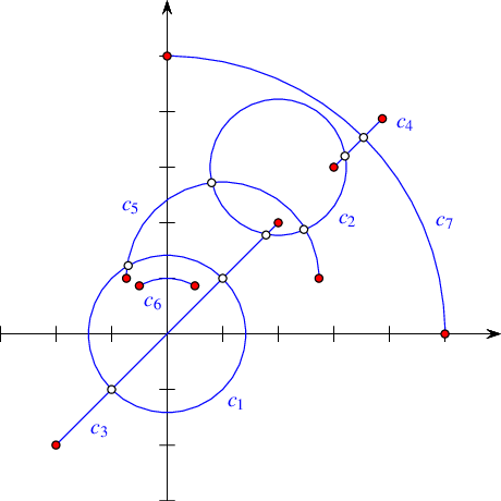
Figure 35.27 An arrangement of two full circles, two line segments, and three circular arcs as constructed in Arrangement_on_surface_2/circular_arcs.cpp. Endpoints are drawn as red disks and intersection points are drawn as rings.
The following example demonstrates the usage of the various construction methods for circular arcs and line segments. The resulting arrangement is depicted in Figure 35.27. Note the usage of the constructor of CoordNT(alpha, beta, gamma), which creates a degree- \(2\) algebraic number whose value is \(\alpha +
\beta\sqrt{\gamma}\).
File Arrangement_on_surface_2/circular_arcs.cpp
It is also possible to construct \(x\)-monotone curve objects that represent \(x\)-monotone circular arcs or line segments using similar constructors. (Full circles are not \(x\)-monotone.)
The traits class-template Arr_circular_line_arc_traits_2<CircularKernel> offered by the arrangement package also handles circular arcs and line segments. It is an alternative to the Arr_circle_segment_traits_2<Kernel> class-template. These two class templates, while serve similar purposes, are based on different concepts, and posses different characteristics. You are encouraged to experiment with both, compare their performance, and use the most suitable for your case.
A conic curve is an algebraic curve of degree 2. Namely, it is the locus of all points \((x,y)\) satisfying the equation \(c:\ r x^2 + s y^2 + t xy + u x + v y + w = 0\), where the six coefficients \(\langle r, s, t, u, v, w \rangle\) completely characterize the curve. The sign of the expression \(\Delta_{c} = 4 r s - t^2\) determines the type of curve:
If \(\Delta_{c} > 0\), the curve is an ellipse. A circle is a special case of an ellipse, where \(r = s\) and \(t = 0\).
If \(\Delta_{c} = 0\), the curve is a parabola—an unbounded conic curve with a single connected branch. When \(r = s = t = 0\) we have a line, which can be considered as a degenerate parabola.
If \(\Delta_{c} < 0\), the curve is a hyperbola. That is, it comprises of two disconnected unbounded branches.
The Arr_conic_traits_2<RatKernel, AlgKernel, NtTraits> class template is capable of handling only bounded arcs of conic curves, referred to as conic arcs. A conic arc \(a\) may be either (i) a full ellipse, or (ii) defined by the tuple \(\langle \kappa,
p_s, p_t, o \rangle\), where \(\kappa\) is a conic curve and \(p_s\) and \(p_t\) are two points on \(c\) (namely \(\kappa(p_s) = \kappa(p_t) = 0\)) that define the source and target of the arc, respectively. The arc is formed by traversing \(\kappa\) from the source to the target going in the orientation specified by \(o\), which is typically clockwise or counterclockwise orientation, but may also be collinear in case of degenerate conic conic-curves, namely, lines or pairs of lines.
We always assume that the conic coefficients \(\langle r, s, t, u, v, w \rangle\) are rational. The coordinates of points of intersection between two conic curves with rational coefficients are in general algebraic numbers of degree 4. Namely, they are roots of algebraic polynomials of degree 4. In addition, conic arcs may not necessarily be \(x\)-monotone, and must be split at points where the tangent to the arc is vertical. In the general case such points typically have coordinates that are algebraic numbers of degree 2. Note that as arrangement vertices induced by intersection points and points with vertical tangents are likely to have algebraic coordinates, we also allow the original endpoints of the input arcs \(p_s\) and \(p_t\) to have algebraic coordinates.
The Arr_conic_traits_2<RatKernel, AlgKernel, NtTraits> class template is designed for efficient handling of arrangements of bounded conic arcs. The template has three parameters, defined as follows:
The RatKernel template parameter must be substituted by a geometric kernel whose field type is an exact rational type. It is used to define basic geometric entities (e.g., a line segment or a circle) with rational coefficients. Typically we use one of the standard CGAL kernels, instantiated with the number type NtTraits::Rational (see below).
The AlgKernel template parameter must be substituted by a geometric kernel whose field type is an exact algebraic type. It is used to define points with algebraic coordinates. Typically, we use one of the standard CGAL kernels, instantiated with the number type NtTraits::Algebraic (see below).
The NtTraits template parameter must be substituted by a type that encapsulates all the numeric operations needed for performing geometric computation carried out by the geometric traits class. It defines the Integer, Rational, and Algebraic number-types, and supports several operations on these types, such as conversion between these types, solving quadratic equations, and extracting the real roots of polynomials with integer coefficients. The use of the CORE_algebraic_number_traits class, which is included in the arrangement package, is highly recommended. The traits class-template relies on the multi-precision number types implemented in the Core library and performs exact computations on the number types it defines.
The instantiation of the conic traits class-template is slightly more complicated than the instantiation of the traits classes you have encountered so far. This instantiation is exemplified in the header file arr_conics.h. Note how we first define the rational and algebraic kernels using the number types given by the Core number type traits-class, then use them to define the conic traits class-template. Also note the types defined by the rational kernels, which we need for conveniently constructing conic arcs.
The Arr_conic_traits_2 models the ArrangementTraits_2 and ArrangementLandmarkTraits_2 concepts. Its Point_2 type is derived from AlgKernel::Point_2, while the Curve_2 type represents a bounded, not necessarily \(x\)-monotone, conic arc. The X_monotone_curve_2 type is derived from Curve_2, but its constructors are used only by the traits class. Users should therefore construct only Curve_2 objects and insert them into the arrangement using the insert() function.
Conic arcs are constructible from full ellipses or by specifying a supporting curve, two endpoints, and an orientation. However, several constructors of Curve_2 are available to allow for some special cases, such as circular arcs or line segments. The Curve_2 and the derived X_monotone_curve_2 classes also support basic access functions such as source(), target(), and orientation().
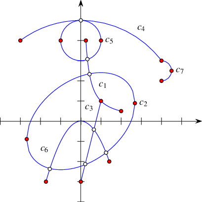
Figure 35.28 An arrangement of mixed conic arcs, as constructed in conics.cpp
The following example demonstrates the usage of the various constructors for conic arcs. The resulting arrangement is depicted in Figure 35.28. Especially noteworthy are the constructor of a circular arc that accepts three points, the constructor of a conic arc that accepts five points, and the constructor that allows specifying approximate endpoints, where the exact endpoints are given explicitly as intersections of the supporting conic with two other conic curves. The approximate endpoints are used to select the specific exact endpoints out of all intersection points of the pair of curves (the supporting conic curve and the auxiliary conic curve). Also note that as the preconditions required by some of these constructors are rather complicated (see the Reference Manual for the details), a precondition violation does not cause the program to terminate—instead, an invalid arc is created. The call a.is_valid() verifies the validity of the arc \(a\). Naturally, inserting invalid arcs into an arrangement is not allowed, so the validity of an arc should be checked once it is constructed.
File Arrangement_on_surface_2/conics.cpp
The types common to the example programs that use the Arr_conic_traits_2 class template are listed below and defined in the header file arr_conics.h.
Figure 35.29 An arrangement of a circular arc and an hyperbolic arc, as constructed in Arrangement_on_surface_2/conic_multiplicities.cpp.
The last example in this section demonstrates how the conic-traits class can handle intersection points with multiplicity. The resulting arrangement is depicted in Figure 35.29. The supporting curves of the two arcs, a circle centered at \((0,\frac{1}{2})\) with radius \(\frac{1}{2}\), and the hyperbola \(y = \frac{x^2}{1-x}\),This curve can also be written as \(c: x^2 + xy - y = 0\). It is a hyperbola since \(\Delta_{c} = -1\). intersect at the origin such that the intersection point has multiplicity \(3\) (note that they both have the same horizontal tangent at \((0,0)\) and the same curvature \(1\)). In addition, they have another intersection point at \((\frac{1}{2},\frac{1}{2})\) of multiplicity \(1\).
File Arrangement_on_surface_2/conic_multiplicities.cpp
A rational function is given by the equation \(y = \frac{P(x)}{Q(x)}\), where \(P\) and \(Q\) are polynomials of arbitrary degrees. In particular, if \( Q(x) = 1\), then the function is simply a polynomial function. A bounded rational arc is defined by the graph of a rational function over some interval \([x_{\rm min}, x_{\rm max}]\), where \(Q\) does not have any real roots in this interval (thus, the arc does not contain any singularities). However, we may consider functions defined over unbounded intervals, namely, over \((-\infty, x_{\max}]\), \([x_{\min}, \infty)\), or \((-\infty, \infty)\). Rational functions, and polynomial functions in particular, are not only interesting in their own right, they are also useful for approximating more complicated curves and for interpolation; see, e.g., [12] Chapter 3.
Using the Arr_rational_function_traits_2 class template it is possible to construct and maintain arrangements induced by rational arcs. Every instance of the Arr_rational_function_traits_2 class template models the concepts ArrangementTraits_2 and ArrangementOpenBoundaryTraits_2, but it does not model the ArrangementLandmarkTraits_2 concept. It also models the refined concept ArrangementDirectionalXMonotoneTraits_2, which enables Boolean set operations; see Package 2D Regularized Boolean Set-Operations Reference. Note that it is not a model of ArrangementLandmarkTraits_2 concept, so it is impossible to use the landmark point-location strategy with this traits class.
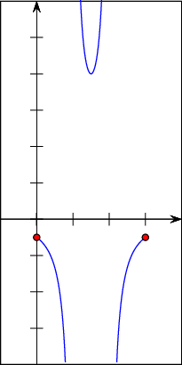
Figure 35.30 An arrangement of an arc of a rational functions that has singularities at \(x = 1\) and at \(x = 2\).
A rational arc is always \(x\)-monotone in the mathematical sense. However, it is not necessarily continuous, as it may have singularities. An arc that has singularities must be split into continuous portions before being inserted into the arrangement. Consider, for example, the rational arc given by the equation \(y =
\frac{1}{(x-1)(2-x)}\) defined over the interval \([0,3]\), as depicted in Figure 35.30. This arc has two singularities, at \(x = 1\) and at \(x = 2\). It is split into three continuous portions defined over the intervals \([0,1)\), \((1,2)\), and \((2,3]\) by the traits operation Make_x_monotone_2. Arbitrary rational functions are represented by the nested type Curve_2 and continuous portions of rational functions are represented by the nested type X_monotone_curve_2. Constructors for both types are provided by the traits in form of functors.
When the Arr_rational_function_traits_2<AlgebraicKernel_d_1> class template is instantiated, the template parameter must be substituted by a model of the AlgebraicKernel_d_1 concept. Models of this concept, such as the Algebraic_kernel_d_1<Coefficient> class template provided by the package Algebraic Foundations are meant to support algebraic functionalities on univariate polynomials of arbitrary degree. See the documentation of the concept AlgebraicKernel_d_1 for more information. A rational function is then represented as the quotient of two polynomials, \(P\) and \(Q\), of type Polynomial_1 nested in every model of the concept AlgebraicKernel_d_1 and in particular in the algebraic-kernel type that substitutes the template parameter AlgebraicKernel_d_1 when the traits class-template is instantiated. Such a rational function is constructible from a single polynomial \(P\) (with \(Q(x) = 1\)), or from two polynomials \(P\) and \(Q\). The type of the polynomial coefficients, namely Coefficient, and the type of the interval bounds, namely Bound, are also nested in the algebraic-kernel type. If an instance of the Algebraic_kernel_d_1<Coefficient> class template is used, for example, as the algebraic-kernel type, the type that substitutes its template parameter is defined as the Coefficient type. This type cannot be algebraic. Moreover, it is recommended that this type is not made rational either, since using rational (as opposed to integral) coefficients does not extend the range of the rational arcs and is typically less efficient.The Algebraic_kernel_d_1 class template uses the types provided by the Polynomial package to define its nested Polynomial_1 type and conveniently expose it to the user. The Bound type, however, can be algebraic. A point of type Point_2 nested in the Arr_rational_function_traits_2 class template is represented by a rational function and its \(x\)-coordinate, which is derived from the type Algebraic_real_1 nested in the algebraic-kernel type. An explicit representation by the nested type Algebraic_real_1 of the \(y\)-coordinate is only computed upon request, as it can be a rather costly operation.
The aforementioned types, Polynomial_1, Coefficient, Bound, and Algebraic_real_1, are conveniently nested in the Arr_rational_function_traits_2 class template among the others and obtained from there in the type definitions used in the examples given in this section and listed below. These types are defined in the header file arr_rat_functions.h.
The constructed rational functions are cached by the traits class. The cache is local to each traits class object. It is therefore necessary to construct curves using only the constructor objects provided by member functions of the traits class. Moreover, a curve must only be used by the traits class object that was used to construct it. The cache is automatically cleaned up from time to time. The amortized clean up costs are constant. In addition, there is also a separate member function that cleans up the cache upon request.
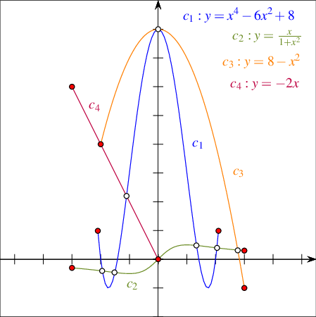
Figure 35.31 An arrangement of four arcs of rational functions, as constructed in Arrangement_on_surface_2/rational_functions.cpp.
The following example demonstrates the construction of an arrangement induced by rational arcs depicted in Figure 35.31. It uses constructors both for polynomial arcs and for rational arcs.
File Arrangement_on_surface_2/rational_functions.cpp
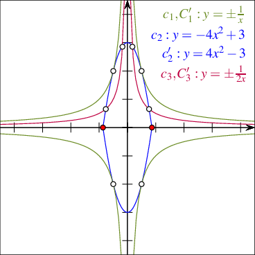
Figure 35.32 An arrangement of six arcs of rational functions, as constructed in Arrangement_on_surface_2/unbounded_rational_functions.cpp.
The following example demonstrates the construction of an arrangement of six rational arcs, four unbounded arcs and two bounded ones, as depicted in Figure 35.32. Note the usage of the constructors of an entire rational function and of an infinite "ray" of such a function. Also observe that the hyperbolas \(y = \pm\frac{1}{x}\) and \(y = \pm\frac{1}{2x}\) never intersect, although they have common vertical and horizontal asymptotes, so very "thin" unbounded faces are created between them:
File Arrangement_on_surface_2/unbounded_rational_functions.cpp
The curve constructors have an additional advantage. They conveniently enable the provision of two polynomials that define a rational arc using rational coefficients. For example, let \(P\) and \(Q\) denote two polynomials with integral coefficients that define a rational arc of interest, and let \(P'\) and \(Q'\) denote two polynomials with rational coefficients that define the same rational arc; that is, the quotients \(P/Q\) and \(P'/Q'\) are identical. You can construct the rational arc providing the coefficients of \(P'\) and \(Q'\) to the constructor. In this case the constructor normalizes the coefficients and generates the desired polynomials \(P\) and \(Q\). To this end, the curve constructors of both types, namely Curve_2 and X_monotone_curve_2, have operators that accept ranges of polynomial coefficients as well as polynomials. The coefficients in a given range must be in the order of the degrees of the corresponding variables starting from the constant term.
A planar Bézier curve \(B\) is a parametric curve defined by a sequence of control points \(p_0, \ldots, p_n\) as follows:
\begin{eqnarray*} B(t) = \left(X(t), Y(t)\right) = \ccSum{k=0}{n}{p_k \cdot \frac{n!}{k! (n-k)!} \cdot t^k (1-t)^{n-k}}\ . \end{eqnarray*}
where \(t \in [0, 1]\). The degree of the curve is therefore \(n\); namely, \(X(t)\) and \(Y(t)\) are polynomials of degree \(n\). Bézier curves have numerous applications in computer graphics and solid modeling. They are used, for example, in free-form sketches and for defining the true-type fonts.
Using the Arr_Bezier_curve_traits_2<RatKernel, AlgKernel, NtTraits> class template you can construct and maintain arrangements induced by Bézier curves (including self-intersecting Bézier curves) of arbitrary degree. The curves are given by rational control points, that is, a sequence of objects of the RatKernel::Point_2 type. (In general, a sequence of \(n+1\) control points define a Bézier curve of degree \(n\).) The three types that substitute the template parameters RatKernel, AlgKernel, and NtTraits, respectively, when the traits is instantiated must fulfill the same requirements of the corresponding types used to instantiate the Arr_conic_traits_2 class template. Here, the use of the CORE_algebraic_number_traits class is also recommended with Cartesian kernels instantiated with the Rational and Algebraic number types defined by this class. The examples given in this manual use the type definitions listed below. These types are defined in the header file arr_Bezier.h.
As mentioned above, we assume that the coordinates of all control points that define a Bézier curve are rational numbers, so both \(X(t)\) and \(Y(t)\) are polynomials with rational coefficients. The intersection points between curves are, however, algebraic numbers, and their exact computation is time-consuming. The traits class therefore contains a layer of geometric filtering that performs all computations in an approximate manner whenever possible. Thus, it resorts to exact computations only when the approximate computation fails to produce an unambiguous result. Most arrangement vertices are therefore associated with approximated points. You cannot access the coordinates of such points as algebraic numbers. However, access to the approximate coordinates is possible. See the Reference Manual for the exact interface of the Point_2, Curve_2, and X_monotone_curve_2 types defined by the traits class.
Every instance of the Arr_Bezier_curve_traits_2 class templates models the concept ArrangementTraits_2 (but it does not model the ArrangementLandmarkTraits_2 concept). It also models the refined concept ArrangementDirectionalXMonotoneTraits_2, which enables Boolean set operations; see Package 2D Regularized Boolean Set-Operations Reference.
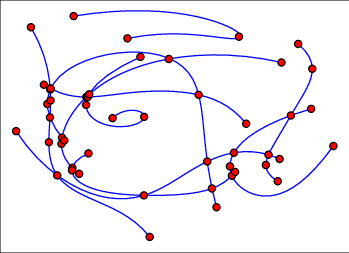
Figure 35.33 An arrangement of ten Bézier curves of degree \(5\), as constructed in Arrangement_on_surface_2/Bezier_curves.cpp.
The following example reads a set of Bézier curves from an input file, where each file is specified by an integer stating its number of control points, followed by the sequence of control points given as integer or rational coordinates. By default, the program uses the Bezier.dat file, which contains ten curves of degree \(5\) each; their resulting arrangement is depicted in Figure 35.33.
File Arrangement_on_surface_2/Bezier_curves.cpp
The traits class, namely Arr_algebraic_segment_traits_2, is based on the Algebraic_kernel_d_1 class template, which models the algebraic-kernel concept AlgebraicKernel_d_1; see Section A Traits Class for Arcs of Rational Functions. The traits class handles (i) algebraic curves and (ii) continuous (weakly) \(x\)-monotone segments of algebraic curves, which, however, are not necessarily maximal. (A formal definition is given below.) Observe that non- \(x\)-monotone segments are not supported. Still, it is the traits class that supports the most general type of curves among the traits classes included in the package.
Recall that an algebraic curve \(c\) in the plane is defined as the (real) zero set of a bivariate polynomial \(f(x,y)\). The curve is uniquely defined by \(f\), although several polynomials might define the same curve. We call \(f\) a defining polynomial of \(c\).
A formal definition of (weakly) \(x\)-monotone segments of algebraic curves follows. A point \(p\) on a curve \(c_f \subset \mathbb{R}^2\) (with defining polynomial \(f\)) is called semi-regular if, locally around \(p\), the curve \(c_f\) can be written as a function graph of some continuous function in \(x\) or in \(y\). (We also say that \(p\) is parameterizable in \(x\) or \(y\), respectively.) The only two cases of non-semi-regular points are isolated points and self-intersections. A segment of a curve in this context is a closed and continuous point set such that each interior point is semi-regular. It follows that a segment is either vertical or a closed connected point set, with all interior points parameterizable in \(x\).
Every instance of the Arr_algebraic_segment_traits_2<Coefficient> class template models the ArrangementTraits_2 and ArrangementOpenBoundaryTraits_2 concepts (but it does not model the ArrangementLandmarkTraits_2 concept). The template argument Coefficient determines the type of the scalar coefficients of the polynomial. Currently supported integral number types are Gmpz, leda_integer, and CORE::BigInt. This is reflected in the statements included in the header file integer_type.h, the listings of which are omitted here. This header file is used by the two example programs listed in this section. The template parameter Coefficient can be substituted in addition by an instance of the Sqrt_extension<A,B> class template, where the template parameters NT and Root are substituted in turn by one of the integral number types above. Finally, the template parameter Coefficient can be substituted also by a rational number type, where the type of the numerator and denominator is one of the types above.
The type Curve_2 nested in the Arr_algebraic_segment_traits_2 class template defines an algebraic curve. An object of this type can be constructed by the Construct_curve_2 functor also nested in the class template. Its function operator accepts as an argument an object of type Polynomial_2, nested as well in the traits class-template. The type Polynomial_2 models the concept Polynomial_d. An object of the nested type Polynomial_2 represents a bivariate polynomial. It can be constructed in a few convenient ways, some are exemplified by the programs listed below. Consult the reference guide for the complete set of options.
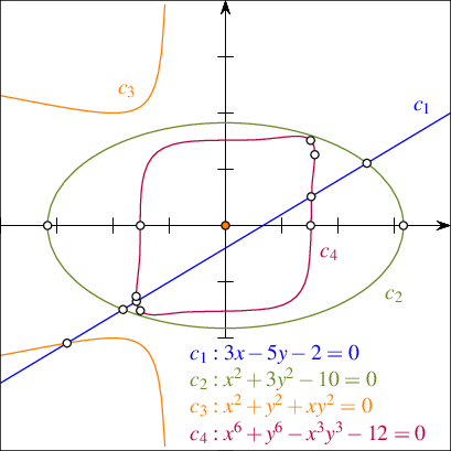
Figure 35.34 An arrangement of algebraic curves of degrees \(1\), \(2\), \(3\), and \(6\), as constructed in Arrangement_on_surface_2/algebraic_curves.cpp.
The following examples computes the arrangement depicted in in Figure 35.34. The arrangement is induced by four algebraic curves, \(c_1\), \(c_2\), \(c_3\), and \(c_4\), of degrees \(1\), \(2\), \(3\), and \(6\), respectively. For each curve the defining polynomial is constructed first. Then, the algebraic curve is constructed using the Construct_curve_2 functor. Finally, the curve is inserted into the arrangement.
File Arrangement_on_surface_2/algebraic_curves.cpp
The Arr_algebraic_segment_traits_2 class template carries state to expedite some of its computations. Thus, it is essential to have only one copy of the traits object during the life time of a program that utilizes this traits class. To this end, the example above uses the constructor of the Arrangement_2 data structure that accepts the traits object as input. Carrying state is not a unique property of the Arr_algebraic_segment_traits_2 class template; it is common to many traits classes, especially to traits classes that handle algebraic curves. Therefore, as a general rule, if your application requires direct access to a traits object, define it locally, and pass it to the constructor of the Arrangement_2 data structure to avoid the construction of a duplicate traits-class object.
A weakly \(x\)-monotone segment of an algebraic curve is represented by the X_monotone_curve_2 type nested in the traits class-template. You can construct such segments in two ways as follows: (i) using the Make_x_monotone_2 functor or (ii) using the Construct_x_monotone_segment_2 functor. Both functors are nested in the traits class-template. The former is required by the concept ArrangementTraits_2 our traits class models; see Section Supporting Arbitrary Curves. The latter enables the construction of individual segments. The X_monotone_curve_2 type represents weakly \(x\)-monotone segments of a curve; however, for technical reasons, segments may need to be further subdivided into several sub-segments, called terminal segments. Therefore, Construct_x_monotone_segment_2 constructs a sequence of X_monotone_curve_2 objects, whose union represents the desired weakly \(x\)-monotone segment. The function operator of the Construct_x_monotone_segment_2 functor accepts as arguments the underlying algebraic curve, the leftmost point of the segment, the rightmost point of the segment, and an output iterator associated with a container of output terminal segments. The function operator is overloaded. In addition to the variant above, there is one that accepts the underlying algebraic curve, a single point \(p\), an enumerator that delimits the segment, and an output iterator. It returns the maximal \(x\)-monotone segment that contains \(p\). The enumerator specifies whether \(p\) is interior to the returned segment, its left endpoint, or its right endpoint. The third variant accepts only two delimiting points and an output iterator. It constructs line segments.
The subdivision terminal segments is due to the internal representation of \(x\)-monotone segments, which is based on a vertical decomposition. We assume the defining polynomial \(f\) of the curve \(c\) to be square-free. That is, it contains no divisor \(g^2\) of total degree greater than zero. We define a (complex) critical point \(p\in\mathbb{C}^2\) by
\[ f(p)=0=\frac{\partial f}{\partial y}(p). \]
An \(x\)-coordinate \(\alpha\in\mathbb{R}\) is critical either if some critical point has \(x\)-coordinate \(\alpha\), or if the leading coefficient of \(f\), considered as a polynomial in \(y\), vanishes. In particular, vertical lines and isolated points of \(c\) can only take place at critical \(x\)-coordinates. Between two consecutive critical \(x\)-coordinates the curve decomposes into a finite number of \(x\)-monotone segments (the same holds to the left of the leftmost, and to the right of the rightmost critical \(x\)-coordinate). The type X_monotone_curve_2 is only capable of representing such segments (and sub-segments of them). Formally, a terminal segment is either a vertical line-segment or a segment of an \(x\)-monotone curve whose \(x\)-range does not contain critical points in its interior. See Figure 35.35 for an example of a quartic curve and its decomposition into terminal segments. Notice that six vertices split the curve into \(x\)-monotone segments, and four additional vertices further split the corresponding \(x\)-monotone segments into terminal segments.
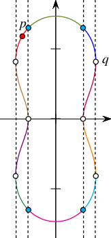
The critical \(x\)-coordinates of an algebraic curve (dashed lines), and its decomposition into terminal segments (in different colors). The segment from \(p\) to \(q\) consists of the union of three terminal segments.
The type Algebraic_real_1 must be defined by any model of the AlgebraicKernel_d_1 concept. The traits class-template Arr_algebraic_segment_traits_2 exploits an instance of the Algebraic_kernel_d_1 class template, which models the concept AlgebraicKernel_d_1. The exploited instance is nested in the traits class-template. You can use this model to create algebraic numbers as roots of univariate polynomials, and process them, for instance, compare them or approximate them to any precision. See the documentation of the concept AlgebraicKernel_1 for more information. Coordinates of points are represented by the type Algebraic_real_1 nested in the traits class-template. This type is defined as the corresponding type nested in the instance of Algebraic_kernel_d_1.
You can construct an object of type Point_2 using the Construct_point_2 functor nested in the traits class-template. Its function operator is overloaded with a couple of variants that accepts the \(x\) and \(y\) coordinates of the point. Their types must be either Algebraic_real_1 or Coefficient. Another efficient variant accepts a triple \((x_0,c,i)\), which identifies the \(i\)-th point (counted from below) in the fiber of \(c\) at the \(x\)-coordinate \(x_0\). The fiber of a curve \(c\) at some \(x\)-coordinate \(x'\) is the set of all points on \(c\) with \(x\)-coordinate \(x'\). Formally, for a curve \(c\) and \(x'
\in \mathbb{R}\), the fiber of \(c\) at \(x'\) is \(c \cap
{(x',b),|,b \in \mathbb{R}}\). In the example depicted in Figure 35.35, if \(x_1\) denotes the \(x\)-coordinate of \(p\), and \(c\) represents the algebraic curve, then \(p\) could be represented by \((x_1,c,3)\). If \(x_2\) is the \(x\)-coordinate of \(q\), then \((x_2,c,1)\) is a valid representation of \(q\). Points are represented internally using the triple described above. Although the \(y\)-coordinate of a point represented by an object of the nested type Algebraic_real_1 can be obtained, we advise caution with that option, since computing an explicit representation of the \(y\)-coordinate can be rather expensive.
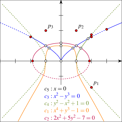
Figure 35.36 An arrangement of algebraic segments (solid lines), as constructed in Arrangement_on_surface_2/algebraic_segments.cpp. The supporting curves are drawn as dashed lines.
The following code exemplifies the method to construct points and the various methods to construct algebraic segments. The computed arrangement is depicted in Figure 35.36.
File Arrangement_on_surface_2/algebraic_segments.cpp
A great circle of a sphere is the intersection of the sphere and a plane that passes through the center point of the sphere. For all pairs of distinct points on the sphere except for antipodal points, there is a unique great circle through the two points. There are infinitely many great circles through antipodal points. The minor arc of a great circle between two points is the shortest spherical-path between them. In this sense, minor arcs are analogous to line segments in Euclidean geometry.
The Arr_geodesic_arc_on_sphere_traits_2<Kernel,X,Y> class template handles arcs of great circles (also known as geodesic arcs) of a unit sphere (centered at the origin in \(\mathbb{R}^3\)). It is a model of the concept ArrangementSphericalBoundaryTraits_2; see Section Supporting Unbounded Curves or Curved Surfaces. An arrangement type (an instance of the template Arrangement_on_surface_2<GeomTraits, TopolTraits>) that uses an instance of this traits class as the geometry traits must use a matching topology traits. Currently, this package provides one template, namely, Arr_spherical_topology_traits_2<GeometryTraits_2, Dcel> an instance of which can be used as the topology traits.
The unit sphere is defined over a parameter space \(\Phi =
[\tau,2\pi+\tau] \times [-\frac{\pi}{2}, \frac{\pi}{2}]\), where \(\tau = \arctan(X, Y)\). By default, \(X = -1, Y = 0\), which implies \(\tau = -\pi\), which implies a default parameterization \(\Phi = [-\pi, \pi] \times [-\frac{\pi}{2}, \frac{\pi}{2}]\). The equator curve, for example, is given by \(\gamma(t) = (2t\pi + \tau,
0)\), for \(t \in [0,1]\). The surface is given by \(\phi_S(\alpha,\beta) = (\cos \alpha \cos \beta, \sin \alpha \cos
\beta, \sin \beta)\); see Section Arrangements on Curved Surfaces for more details. This parameterization induces two contraction points \((0,0,-1) = \phi_S(\alpha,-\frac{\pi}{2})\) and \((0,0,1) =
\phi_S(\alpha,\frac{\pi}{2})\), for all \(\alpha\), referred to as the south and north poles, respectively, and an identification curve \(\{\phi_S(\alpha,\beta)\,|\,-\frac{\pi}{2} \leq \beta \leq
\frac{\pi}{2}\}\), as \(\phi_S(\pi,\beta) = \phi_S(2\pi +
\tau,\beta)\) for all \(\beta\). When \(\tau = -\pi\) (the default), the identification curve coincides with the opposite Prime (Greenwich) Meridian. In other words, the left and right boundary sides of the parameter space are identified and the top and bottom boundary sides are contracted. The arguments that substitute the template parameters X and Y when Arr_geodesic_arc_on_sphere_traits_2<Kernel, X, Y> is instantiated determine the value of \(\tau\). Essentially, overriding their default values rotates the identification curve about the vertical axes of the image coordinate system (that is, the sphere coordinate system). These arguments must be integral values. They define a not-necessarily normalized vector \((x,y)\) in the \(xy\)-plane in the image coordinate system, that bisects the identification curve. The explicit expression for the surface above is not used at all in the implementation of the traits. Indeed, all the required geometric operations listed in the traits concept are implemented using only rational arithmetic.
The following example constructs an arrangement induced by 12 arcs of great circles embedded in the sphere. The arrangement is depicted in Figure 35.37.
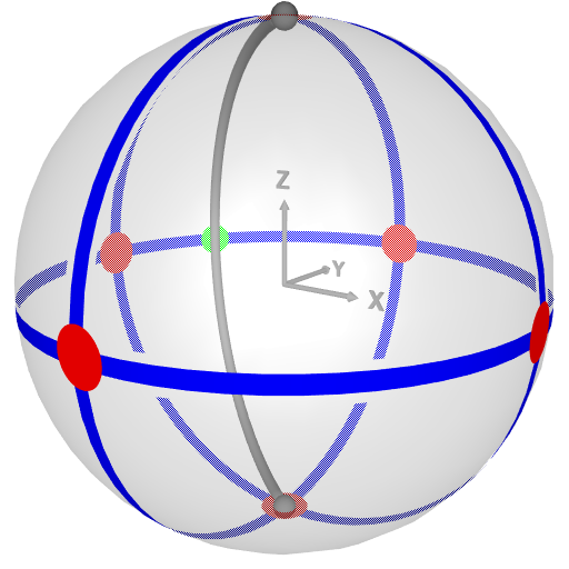
Figure 35.37 An arrangement induced by 12 arcs of great circles, as constructed in Arrangement_on_surface_2/spherical_insert.cpp. The number of vertices, edges, and faces of the arrangement is 7, 13, and 8, respectively. The intersection of the curve \((-1,0,0),(0,1,0)\) with the identification curve induces a vertex at \((\frac{-11}{\sqrt{11^2+7^2}},\frac{7}{\sqrt{11^2+7^2}},0)\) drawn in green. The north and south poles are drawn as little spheres. The identification curve is drawn as a gray tube.
File Arrangement_on_surface_2/spherical_insert.cpp
Use the Arr_geodesic_arc_on_sphere_traits_2::Construct_point_2, Arr_geodesic_arc_on_sphere_traits_2::Construct_x_monotone_curve_2, and Arr_geodesic_arc_on_sphere_traits_2::Construct_curve_2 functors to construct a point, an \(X\)-monotone curve and a curve objects, respectively. Observe that an \(X\)-monotone curve cannot intersect the identification curve in its interior. A curve can be constructed from either (i) two endpoints, (ii) two endpoints and a normal, or (iii) a normal. The two endpoints determine the plane. The normal determines the orientation of the plane and the final arc (whether it is the minor arc or the major arc). If the normal is not provided, the minor arc is constructed. If a curve is constructed and only the normal is provided a full great circle is constructed. If an \(X\)-monotone curve is constructed and only the normal is provided an arc that resembles a full circle is constructed; this arc has one endpoint that lies on the identification curve; this point is considered both the source and target (and also the left and right) point of the arc. See Figure 35.38 for an illustration of the right-hand rule, which depicts the relation between the arc and the normal.
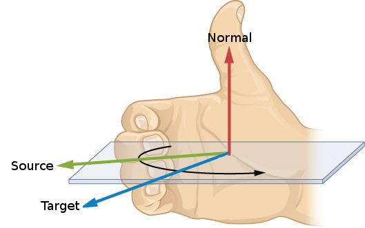
Figure 35.38 To use the right hand rule, point your right thumb in the direction of the normal and curl your fingers in the direction of the arc starting with source endpoint and ending at the target endpoint.
Decorator is a structural pattern that allows adding new behaviors to objects by placing them inside special wrapper objects, called decorators. One type of decorators attaches auxiliary data to the geometric objects handled by the original traits. Another type enables the retrieval of debugging and informative metadata.
Geometric traits-class decorators allow you to attach auxiliary data to the geometric objects (curves and to points). The data is automatically manipulated by the decorators and distributed to the constructed geometric entities. Additional information can alternatively be maintained by extending the vertex, halfedge, or face types provided by the DCEL class used by the arrangement; see Section Extending the DCEL for details. In many cases, however, it is convenient to attach the data to the curve itself, exploiting the automatic proliferation of the additional data fields from each curve to all its induced subcurves. Moreover, as two halfedges are associated with a single curve, storing the data once in the curve record either saves space or avoids an indirect access from one halfedge to its twin.
The 2D Arrangements package includes a traits-class decorator used to attach a data field to curves and to \(x\)-monotone curves. It is a class template named Arr_curve_data_traits_2<BaseTraits, XMonotoneCurveData, Merge, CurveData, Convert> parameterized by a base-traits class, which must be substituted by one of the geometric traits models described in the previous subsections or with a user-defined traits model, when the decorator is instantiated. The curve-data decorator derives from the base-traits class, and in particular inherits its Point_2 type. The remaining nested types are defined as follows:
Curve_2 is derived from the basic BaseTraits::Curve_2 class, extending it by an extra field of type CurveData.
X_monotone_curve_2 is derived from the basic BaseTraits::X_monotone_curve_2 class, extending it by an extra field of type XMonotoneCurveData, which must model the concepts CopyConstructible, EqualityComparable, and DefaultConstructible. The latter ensures that every instance of the class template Arr_curve_data_traits_2 obtained by substituting the BaseTraits template parameter with a model of the ArrangementLandmarkTraits_2 concept models the ArrangementLandmarkTraits_2 concept as well
Note that the nested Curve_2 and X_monotone_curve_2 are not the same, even if the BaseTraits::Curve_2 and BaseTraits::X_monotone_curve_2 are (as in the case of the segment-traits class, for example). The extended curve types support the additional methods <Tr, XData, Mrg, CData, Cnv>::Curve_2::data() data() and <Tr, XData, Mrg, CData, Cnv>::Curve_2::set_data() set_data() for accessing and modifying the data field.
You can create an extended curve (or an extended \(x\)-monotone curve) from a basic curve and a curve-data object. When curves are inserted into an arrangement, they may be split, and the decorator handles their data fields automatically as follows:
When a curve is subdivided into \(x\)-monotone subcurves, its data field of type CurveData is converted to an object of type XMonotoneCurveData using the Convert functor. The object is automatically associated with each of the resulting \(x\)-monotone subcurves.
Note that by default, the CurveData type is identical to the XMonotoneCurveData type (and the conversion functor Convert is trivially defined). Thus, the data field associated with the original curve is just duplicated and stored with the \(x\)-monotone subcurves.
When an \(x\)-monotone curve is split into two (typically, when it intersects another curve), the decorator class automatically copies its data field to both resulting subcurves.
When two \(x\)-monotone curves, \(c_1\) and \(c_2\), intersect, the result may include overlapping sections represented as \(x\)-monotone curves. In this case the data fields of \(c_1\) and \(c_2\) are merged into a single XMonotoneCurveData object using the Merge functor, which is supplied as a parameter to the traits class-template. The resulting object is assigned to the data field of the overlapping subcurves.
Merging two \(x\)-monotone curves is allowed only when (i) the two curves are geometrically mergeable—that is, the base-traits class allows to merge them, and (ii) the two curves store the same data field.
Another decorator supported by the 2D Arrangements package is the Arr_consolidated_curve_data_traits_2<BaseTraits, Data> class template. It derives from the Arr_curve_data_traits_2 class template, and it extends the basic type BaseTraits::Curve_2 by a single Data field, and the basic BaseTraits::X_monotone_curve_2 with a set of (distinct) data objects. The Data type must model the concept EqualityComparable to ensure that each set contains only distinct data objects with no duplicates. When a curve with a data field \(d\) is subdivided into \(x\)-monotone subcurves, each subcurve is associated with a set \(S = \{d\}\). In the case of an overlap between two \(x\)-monotone curves \(c_1\) and \(c_2\) with associated data sets \(S_1\) and \(S_2\), respectively, the overlapping subcurve is associated with the consolidated set \(S_1 \cup S_2\).
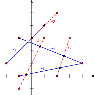
Figure 35.39 An arrangement of six red and blue segments, as constructed in Arrangement_on_surface_2/consolidated_curve_data.cpp. Disks correspond to red-blue intersection points, while circles mark the endpoints of red-blue overlaps.
The following example uses Arr_segment_traits_2 as the base-traits class, attaching an additional color field to the segments using the consolidated curve-data traits class. A color may be either blue or red. Having constructed the arrangement of colored segments, as depicted in Figure 35.39, we detect the vertices that have incident edges mapped to both blue and red segments. These vertices, drawn as black discs in the figure, correspond to red-blue intersection points. We also locate the edge that corresponds to overlap between a red and a blue line segment (its endpoints are also drawn as black discs)
File Arrangement_on_surface_2/consolidated_curve_data.cpp
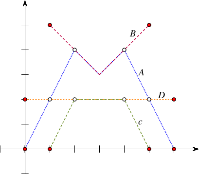
Figure 35.40 An arrangement of four polylines, named A-D, as constructed in Arrangement_on_surface_2/generic_curve_data.cpp.
The following example uses Arr_polyline_traits_2 as the base-traits class, attaching an additional name field to each polyline using the generic curve-data traits class. It constructs an arrangement of four polylines, named \(A\), \(B\), \(c\), and \(D\), as illustrated in Figure 35.40. In the case of overlaps, it simply concatenate the names of the overlapping polylines. At the end of the program the curve associated with the edges that correspond to overlapping polylines are replaced with geometrically equivalent curves, but with different data fields.
File Arrangement_on_surface_2/generic_curve_data.cpp
The third example we give in this section is based on Arrangement_on_surface_2/dual_lines.cpp given in Section Point-Line Duality. It constructs the arrangement of the dual lines for a set of point given in an input file (by default we use coll_points.dat, which contains \(50\) points randomly selected on the grid \([-100,100]\times[-100,100]\); the file contains two distinct triplets of collinear points). Here we use the generic curve-data decorator to attach the index of the primal point to each of the lines. Doing so, we can go over the incident edges of each vertex whose degree is greater than \(4\) and report the subsets of collinear points (if we have a vertex of degree \(d\), we actually need to go over \(\frac{d}{2}\) edges, as each incident line contributes exactly \(2\) edges). Note that in this case the dual line cannot overlap, so we use a dummy merge functor to instantiate the curve-data traits:
File Arrangement_on_surface_2/dual_with_data.cpp
The package provides two traits-class decorators, namely Arr_counting_traits_2<BaseTraits> and Arr_tracing_traits_2<BaseTraits>, that can be used to insert debugging and informative metadata to an output stream. The former is used to count the number of invocations of traits-class functors, and the latter is used to trace these invocations. Note that the constructors of each of these class templates apply perfect forwarding. The counting traits also exports the count of traits-class objects of specific types constructed during the execution of the program. The tracing traits supports filtering of traced functors. The calls traits.enable_trace(id) and traits.disable_trace(id) enables and disables the tracing of a functor identified by id, respectively. A functor is identified by an enumeration. For example, the functor Make_x_monotone_2 is identified by the enumeration Arr_tracing_traits_2::MAKE_X_MONOTONE_OP. The calls traits.enable_all_traces() and traits.disable_all_traces() enables and disables the traces of all functors, respectively. The example program listed below demonstrates the use of both of these metadata decorators.
File Arrangement_on_surface_2/count_and_trace.cpp
A topology traits class encapsulates the definitions of the topological entities and the implementation of the functions that handle these topological entities, used by the Arrangement_on_surface_2<GeometryTraits_2, TopologyTraits> class template and by the peripheral modules. Every topology traits class must model the basic concept ArrangementBasicTopologyTraits. A model of this basic concept holds the (DCEL) data structure used to represent the arrangement cells (i.e., vertices, edges, and facets) and the incidence relations between them. At this point we do not expose the concepts that refine the basic concept. The package contains three topology traits class templates, namely, Arr_bounded_planar_topology_traits_2, Arr_unb_planar_topology_traits_2, and Arr_spherical_topology_traits_2. The first two are internally used to define any instance of the class template Arrangement_2<GeometryTraits_2, Dcel>. In particular, an instance Arrangement_2<Geometry_traits_2, Dcel_> is derived from the instance Arrangement_on_surface_2<Geometry_traits_2,Topology_traits>, where the Topology_traits type is selected based on the provided geometry traits Geometry_traits_2, or more precisely, on the boundary conditions defined by the geometry traits. If all sides of the boundary of the parameter space are closed, the instance Arr_bounded_planar_topology_traits_2<Geometry_traits_2,Dcel_> is selected; otherwise the instance Arr_unb_planar_topology_traits_2<Geometry_traits_2,Dcel_> is selected. The third topology traits serves as a topology traits for an arrangement embedded on a sphere. More precisely, for an arrangement embedded on a sphere defined over a parameter space, the left and right boundary sides of which are identified, and the top and bottom boundary sides are contracted.
Developing applications that use arrangements to solve problems that are a bit more complicated than the problems presented in previous chapters requires the ability to adapt the arrangement data structure to the application needs. One technique to do this is to extend the arrangement with auxiliary, usually non-geometric, data. In this chapter we describe several ways to extend an arrangement data structure.
In some cases it is essential to know exactly what happens inside a specific arrangement object. For example, when a new curve is inserted into an arrangement, it may be necessary to keep track of the faces that are split due to this insertion operation. Other important examples are the point-location strategies that require auxiliary data structures (see Section Point-Location Queries), which must be kept up-to-date when the arrangement changes. The 2D Arrangements package offers a mechanism that uses observers (see [7]). The objective behind this mechanism is to define a one-to-many dependency between objects, so that when one object changes state, all its dependents are notified and updated automatically. The observed object does not know anything about the observers. It merely "publishes" information about changes when they occur. In our case observers can be attached to an arrangement object.
An observer object that observes changes in an arrangement object stores a pointer to the attached arrangement object. It receives notifications about the changes this arrangement undergoes. The observer receives notifications just before a structural change occurs in the arrangement and immediately after such a change takes place. An observer object that observes changes in an arrangement object of type Arrangement must be of a type derived from Arrangement::Observer, which is an alias to Aos_observer<Arrangement_on_surface_2>, where Arrangement_on_surface_2 is the type of the arrangement object or its base type. An instance of Aos_observer<> serves as a base type for other observer classes and defines a set of virtual notification functions, with default empty implementations. You can also use the template alias Arr_observer<Arrangement_2>, where Arrangement_2 is the type of the arrangement object in case it is derived from an instance of the template Arrangement_on_surface_2. The set of functions can be divided into three categories, as follows:
Notifiers of changes that affect the entire topological structure of the arrangement. This category consists of two pairs (before and after) that notify the observer of the following changes:
Pairs of notifiers before and after a local change that occurs in the topological structure. Most notifier functions belong to this category. The relevant local changes include:
A new vertex is constructed and associated with a point.
An edgeThe term "edge" refers here to a pair of twin halfedges. is constructed and associated with an \(x\)-monotone curve.
An edge is split into two edges.
An existing face is split into two faces, as a consequence of the insertion of a new edge.
A hole is created in the interior of a face.
Two holes are merged to form a single hole, as a consequence of the insertion of a new edge.
A hole is moved from one face to another, as a consequence of a face split.
Two edges are merged into one edge.
Two faces are merged into one face, as a consequence of the removal of an edge that used to separate them.
One hole is split into two, as a consequence of the deletion of an edge that used to connect the two components.
A hole is deleted from the interior of a face.
Notifiers about a change caused by a free function; see Section Free Functions for a discussion on the free functions. This category consists of a single pair of notifiers, namely before_global_change() and after_global_change(). Neither of these functions is invoked by methods of the Arrangement_2 class template. Instead, they are called by the free functions themselves. It is implied that no point-location queries (or any other queries for that matter) are issued between the call to before_global_change() and the call to after_global_change().
See the Reference Manual for a detailed specification of the Aos_observer class template and the prototypes of all notification functions.
Each arrangement object stores a list of pointers to Aos_observer objects. This list may be empty, in which case the arrangement does not have to notify any external class on the structural changes it undergoes. If, however, there are observers associated with the arrangement object, then whenever one of the structural changes listed in the first two categories above is about to take place, the arrangement object performs a forward traversal on this list and invokes the appropriate function of each observer. After the change takes place the observer list is traversed backward (from tail to head), and the appropriate notification function is invoked for each observer.
Concrete arrangement-observer classes should inherit from Aos_observer. When an observer is constructed, it is attached to a valid arrangement supplied to the observed constructor, or alternatively the observer can be attached to the arrangement at a later time. When this happens, the observer object inserts itself into the observer list of the associated arrangement and starts receiving notifications whenever this arrangement changes thereafter. Subsequently, the observer object unregisters itself by removing itself from this list just before it is destroyed. Most concrete observer-classes do not need to use the full set of notifications. Thus, the bodies of all notification methods defined in the base class Aos_observer are empty. A concrete observer that inherits from Aos_observer needs to override only the relevant notification methods. The remaining methods are invoked when corresponding changes occur, but they do nothing.
The trapezoidal map RIC and the landmark point-location strategies both use observers to keep their auxiliary data structures up-to-date. In addition, you can define your own observer classes, inheriting from the base observer class and overriding the relevant notification functions, as required by their applications.
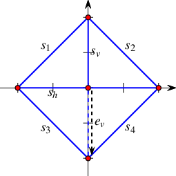
Figure 35.41 An arrangement of six line segments, as constructed in Arrangement_on_surface_2/observer.cpp. The halfedge \(e_v\) (dashed) is eventually removed, so that the final arrangement consists of four faces (one unbounded and three bounded ones).
The following example shows how to define and use an observer class. The observer in the example responds to changes in the arrangement faces. It prints a message whenever a face is split into two due to the insertion of an edge and whenever two faces merge into one due to the removal of an edge. The layout of the arrangement is depicted in Figure 35.41; it comprises six line segments and eight edges (the horizontal segment \(s_h\) and the vertical segment \(s_v\) induce two edges each). The halfedge \(e_v\) is induced by the vertical segment \(s_v\). First, it is associated with the (entire) segment, as obtained by the insert() function; see Line 40 in the code excerpt below. After the insertion of \(s_h\) (see Line 41) the halfedge is split. After the split \(e_v\) (drawn dashed in the figure) is associated with the lower split curve. Eventually, it is removed (along with its twin halfedge). Note the face-split notifications that are invoked as a consequence of the insertion of \(s_v\) and \(s_h\) and the face-merge notification that is invoked as a consequent of the removal of \(e_v\).
File Arrangement_on_surface_2/observer.cpp
Observers are especially useful when the DCEL records are extended and store additional data-fields, since they help update this data stored in these fields, as the following sections reveal.
For many applications of the 2D Arrangements package it is necessary to store additional information (perhaps of non-geometric nature) with the arrangement features. Vertices are associated with Point_2 objects and edges (halfedge pairs) are associated with X_monotone_curve_2 objects, both defined by the traits class. Extending the geometric traits-class types by using a traits-class decorator, as explained in Section Traits-Class Decorators, might be a sufficient solution for some applications. However, the DCEL faces are not associated with any geometric object, so traits-class decorators cannot help here. Extending the DCEL face records comes in handy is such cases. As a matter of fact, it is possible to conveniently extend all DCEL records (namely vertices, halfedges, and faces), which is advantageous for some applications.
All examples presented so far use the default DCEL; namely, they employ the Arr_default_dcel<Traits> instance. This is done implicitly, as this instance of the Arr_default_dcel class template serves as the default parameter for the Arrangement_2 class template; see Section The Arrangement Class Template. The default DCEL class associates points with vertices and \(x\)-monotone curves with halfedges, but nothing more. In this section we show how to use alternative DCEL types to extend the desired DCEL records.
The Arr_face_extended_dcel<Traits, FaceData> class-template is used to associate auxiliary data field of type FaceData to each face record in the DCEL. When the Arrangement_2<Traits,Dcel> class template is instantiated, substituting the DCEL parameter with an instance of this class template, the interface of the nested Face type is extended with the access function data() and with the modifier set_data(). Using these extra functions it is straightforward to access and maintain the auxiliary face-data field.
Note that the extra data-fields must be maintained by the user application. User may choose to construct their arrangement, and may only then go over the faces and store data in the appropriate data-fields of the arrangement faces. However, in some cases the face data can only be computed when the face is created (split from another face or merged with another face). In such cases one can use an arrangement observer tailored for this task, which receives updates whenever a face is modified and sets its data field accordingly.
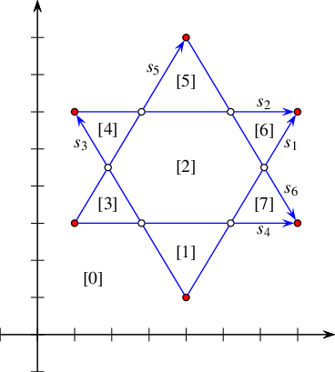
Figure 35.42 An arrangement of six line segments, as constructed in Arrangement_on_surface_2/face_extension.cpp and Arrangement_on_surface_2/dcel_extension.cpp (in Arrangement_on_surface_2/dcel_extension.cpp we treat the segments as directed, so they are drawn as arrows directed from the source to the target). The indices associated with the halfedges in Arrangement_on_surface_2/face_extension.cpp are shown in brackets.
The next example constructs an arrangement that contains seven bounded faces induced by six line segments, \(s_1, \ldots, s_6\), as shown in Figure 35.42. An observer gets notified each time a new face \(f\) is created, and it associates \(f\) with a running index, where the index of the unbounded face is 0. As a result, the faces are numbered according to their creation order, These numbers are shown in brackets, and their order can easily be verified by examining the insertion order of the segments.For simplicity, the particular observer used must be attached to an empty arrangement. It is not difficult however to modify the program to handle the general case of attaching a similar observer to a non-empty arrangement.
File Arrangement_on_surface_2/face_extension.cpp
As you continue to use arrangements to solve various problems you will find out that the ability to extend the face records is crucial. Perhaps less common, but also important to satisfy, is the need to extend the vertex and halfedge records as well. The Arr_extended_dcel<Traits, VertexData, HalfedgeData, FaceData> class-template is used to associate auxiliary data fields of types VertexData, HalfedgeData, and FaceData with DCEL vertex, halfedge, and face record types, respectively. When the Arrangement_2<Traits,Dcel> class template is instantiated, substituting the Dcel parameter with an instance of this DCEL class-template, the interfaces of the nested types Vertex, Halfedge, and Face are extended with the access function data() and with the modifier set_data().
The next example shows how to use a DCEL with extended vertex, halfedge, and face records. In this example each vertex is associated with a color, which is either blue, red, or white, depending on whether the vertex is isolated, represents a segment endpoint, or represents an intersection point. (Notice that the coloring rules suggested here apply only to non-degenerate arrangements, where the sets of isolated points, curve endpoints, and intersection points are mutually exclusive.) In this example segments are treated as directed objects. Each halfedge is associated with Boolean flag indicating whether its direction is the same as the direction of its associated segment. Each face is also extended to store the size of its outer boundary, that is, the number of halfedges along its outer boundary.
The constructed arrangement, depicted in Figure 35.42, is similar to the arrangement constructed in the previous example. In this case, however, we do not use an observer; instead, all auxiliary data-fields are set after the construction phase. Also note that the data fields are properly maintained when the arrangement is copied to another arrangement object.
File Arrangement_on_surface_2/dcel_extension.cpp
The various DCEL classes presented in this section are well suited for most applications based on the 2D Arrangements package. They are all defined using helper constructs, and in particular the base DCEL class-template Arr_dcel_base}. However, there are cases where special requirements, not addressed by these DCEL classes, are needed. In such cases you may explicitly extend the base DCEL class-template, as described in the next paragraph, or implement your own DCEL class from scratch and use the resulting DCEL to instantiate the Arrangement_2 class template. In any case such a class must model the concept ArrangementDcel or its refinement ArrangementDcelWithRebind. The latter requires a rebind struct template, which implements a policy-clone idiom. Here, the DCEL class is the policy class and the rebind member template struct is used to pass a different traits type parameter to the policy class template.
In some cases you may want to extend a certain feature type with several fields. You can gather all these fields (and perhaps methods that access and retrieve these fields) in a single construct, and substitute the appropriate parameter of the class template Arr_extended_dcel<Traits, VertexData, HalfedgeData, FaceData> with this construct. Naturally, you can define three constructs, one for each feature type, and substitute all the three corresponding template parameters appropriately. For example, consider an arrangement that represents a map where features of the same type represent different cartographic entities, e.g., an edge represents a road, a river, or a railway. We would like to associate two strings with each feature, namely, the name and the type of the feature. Following the solution above, accessing or retrieving a specific field will always require an indirection through one of the member functions set_data() and data(). While this indirection is typically resolved at compile time, and thus has no negative effect on the running time of the generated code, it may have some implication on the space consumption due to compiler padding.Compilers add pad bytes into user-defined constructs to comply with alignment restrictions imposed by target microprocessors. Moreover, the code may look cumbersome.
The extended DCEL class that addresses the problem raised above is listed below. Here, each feature type is explicitly extended with two strings, namely, name and type, eliminating the data constructs.
Assume that we are given two geographic maps represented as arrangements, with some data objects attached to their faces, representing some geographic information—for instance, a map of the annual precipitation in some country and a map of the vegetation in the same country—and you are asked to locate, for example, places where there is a pine forest and the annual precipitation is between 1,000mm and 1,500mm. Overlaying the two maps may help you figure out the answer. Computing the overlay of two two-dimensional arrangements is also useful for supporting Boolean set operations on polygons or general polygons; see e.g., [2]).
Formally, the map overlay of two two-dimensional subdivisions \(\mathcal{S}_1\) and \(\mathcal{S}_2\) is a two-dimensional subdivision \(\mathcal{S}\), such that there is a face \(f\) in \(\mathcal{S}\) iff there are faces \(f_1\) and \(f_2\) in \(\mathcal{S}_1\) and \(\mathcal{S}_2\), respectively, such that \(f\) is a maximal connected component of \(f_1 \cap f_2\).
The overlay of two given arrangements, conveniently referred to as the "blue" and the "red" arrangements, is implemented as a plane-sweep algorithm employing a dedicated visitor; see Section The Surface-Sweep Algorithm. The \(x\)-monotone curve type is extended with a color attribute (whose value is either blue or red); see Section Traits-Class Decorators. With the help of the extended type unnecessary computations are filtered out while the plane is swept, yielding an efficient process. For example, monochromatic intersections are not computed.
The plane-sweep visitor that concretizes the overlay operation needs to construct a DCEL that properly represents the overlay of two input arrangements. A face in the overlay arrangement corresponds to overlapping regions of the blue and red faces. An edge in the overlay arrangement is due to a blue edge, a red edge, or an overlap of two differently colored edges. An overlay vertex is due to a blue vertex, a red vertex, a coincidence of two differently colored vertices, or an intersection of a blue and a red curve.
The call overlay(arr_r, arr_b, arr_o,
ovl_traits) constructs the arrangement arr_o, which is the overlay of two input arrangement arr_r and arr_b. All three arrangements must use the same geometric primitives. In other words, their types are instances of the Arrangement_2<Traits,Dcel> class template, where the Traits parameter is substituted by three geometry-traits classes, respectively. The geometry-traits classes of the input arrangements must be convertible to the geometry-traits class of the resulting arrangement.It is sufficient that all three geometry-traits classes used to instantiate the three types of arrangements derive from a common ancestor that models the geometry-traits concept. Typically, all three arrangements use the same geometry-traits class.
The overlay() function template is suitable for arrangements that do not store any additional data with their DCEL records; namely, arrangements defined using the default DCEL, which is the instance Arr_default_dcel<Traits>. Typically, the overlay arrangement in this case does not store extra data with its DCEL records as well. (If it does, the additional data-fields cannot be computed by the overlay operation in this case.) The overlay arrangement is equivalent to the arrangement induced by all curves of arr_r and arr_b. Indeed, it is possible to obtain the same result using the standard insertion-operations instead, but, as mentioned above, this is less efficient.
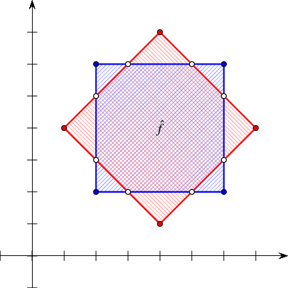
Figure 35.43 Overlaying two simple arrangements of line segments, as done in Arrangement_on_surface_2/overlay.cpp and Arrangement_on_surface_2/face_extension_overlay.cpp. In Arrangement_on_surface_2/face_extension_overlay.cpp the two bounded faces are considered as marked, and the octagonal face which is the intersection of the two marked faces is denoted by \(f_0\).
The next program constructs two simple arrangements; each comprises four line segments that form a square, as depicted in Figure 35.43. The program computes the overlay of the two arrangements. The resulting arrangement has 16 vertices, 24 edges, and 10 faces (including the unbounded one.
File Arrangement_on_surface_2/overlay.cpp
The overlay() function template is overloaded with a variant that accepts four arguments, that is, overlay(arr_r, arr_b, arr_o,
ovl_traits). The type of the ovl_traits additional argument, referred to as the overlay traits, must model the OverlayTraits concept described below. Assume that arr_r is of type Arrangement_2<Traits,Dcel_R>, arr_b is of type Arrangement_2<Traits,Dcel_B>, and the resulting arr_o is of type Arrangement_2<Traits,Dcel_O>. The overlay traits enables the creation of Dcel_O records in the overlay arrangement from the features of Dcel_R and Dcel_B records from the arrangements arr_r and arr_b, respectively.
We distinguish between (i) an overlay of two arrangements that store additional data-fields only with their faces e.g., the geographic-map example given at the beginning of this section) and (ii) an overlay of two arrangements that store additional data fields with all their DCEL records (or at least not only with their faces). The arrangement that results from overlaying two face-extended arrangements typically also stores additional data-fields with its faces. The types of such arrangements, for example, could be instances of the Arrangement_2<Traits,Dcel> class template, where the Dcel parameters are substituted by instances of the Arr_face_extended_dcel class template (see Section Extending the DCEL Faces). The data field that is attached to an overlay face can be computed from the data fields of the two faces (in arr_r and arr_b) that induce the overlay face. Similarly, the arrangement that results from overlaying two arrangements that store additional data fields with all their DCEL records typically also stores additional data-fields with all its DCEL records. The types of such arrangements, for example, could be instances of the Arrangement_2<Traits,Dcel> class template, where the Dcel parameters are substituted by instances of the Arr_extended_dcel class template (see Section Extending All DCEL Records). The data field attached to an overlay feature can be computed from the data fields of the two features (in arr_r and arr_b) that induce the overlay feature.
As mentioned in the previous paragraph, if any of the DCEL records of your arrangements are extended, you can pass a fourth argument to the overlay() call, also referred to as the overlay traits, to control the generation of the extended data in the resulting arrangement. If only the face records are extended, the type of the overlay traits can be an instance of the class template Arr_face_overlay_traits<ArrangementR,ArrangementB,ArrangementO,OverlayFaceData>, which models the concept OverlayTraits. An object of this type operates on face-extended arrangements. When instantiated, the OverlayFaceData parameter must be substituted by a functor that is capable of combining two face-data fields of types ArrangementR::Dcel::Face_data and ArrangementB::Dcel::Face_data and computing the output ArrangementO::Dcel::Face_data object. The face-overlay traits-class uses this functor to properly construct the overlay faces.
The following example shows how to compute the intersection of two polygons using the overlay() function template. It uses a face-extended DCEL type to instantiate the arrangement classes. Each face of the the DCEL is extended with a Boolean flag. A polygon is represented as a marked arrangement face (whose flag is set). The example uses an instance of the Arr_face_overlay_traits<ArrR,ArrB,ArrO,OverlayFaceData> class template as the face-overlay traits class where the OverlayFaceData template parameter is substituted by a functor that simply performs a logical and operation on Boolean flags. As a result, a face in the overlay arrangement is marked only when it corresponds to an overlapping region of two marked faces in the input arrangements. Namely, it is part of the intersection of the two polygons. The example computes the intersection between a parallel-axis square and a congruent square rotated \(45^\circ\). The resulting polygon from the intersection operation is an octagon, which corresponds to the face~ \(\hat{f}\) in the arrangement depicted in Figure 35.43.
File Arrangement_on_surface_2/face_extension_overlay.cpp
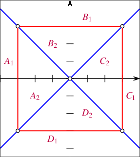
Figure 35.44 Overlaying two arrangements of lines that have unbounded faces, as done in Arrangement_on_surface_2/overlay_unbounded.cpp.
The next example, depicted in Figure 35.44, demonstrates the face overlay of two arrangements that have unbounded faces as well as bounded ones. The first arrangement (blue) is induced by the two lines \(y = x\) and \(y = -x\), which subdivide the plane into four unbounded faces, labeled \(A\), \(B\), \(C\) and \(D\). The second arrangement (red) comprises four line segments that form a square-shaped face indexed \(1\). The unbounded face is indexed 2. When the two arrangements are overlaid, each of the four faces \(A\), \(B\), \(C\) and \(D\) is split into an unbounded face (indexed 2) and a bounded face (indexed 1), so the faces of the resulting arrangement are labeled \(A_1, A_2, \ldots, D_1,
D_2\). boost::lexical_cast is used to cast the integral indices into strings to produce the final labels.
File Arrangement_on_surface_2/overlay_unbounded.cpp
If the red and blue arrangements store additional data-fields with all their DCEL records, and the data associated with the overlay DCEL features should be computed from the red and blue DCEL features that induce it, then an appropriate overlay-traits argument must be passed to the overlay() call. The overlay-traits type models the OverlayTraits concept, which requires the provision of ten functions that handle all possible cases as listed below. Let \(v_r\), \(e_r\), and \(f_r\) denote input red features, i.e., a vertex, an edge, and a face, respectively, \(v_b\), \(e_b\), and \(f_b\) denote input blue features, and \(v\), \(e\), and \(f\) denote output features.
A new vertex \(v\) is induced by coinciding vertices \(v_r\) and \(v_b\).
A new vertex \(v\) is induced by a vertex \(v_r\) that lies on an edge \(e_b\).
An analogous case of a vertex \(v_b\) that lies on an edge \(e_r\).
A new vertex \(v\) is induced by a vertex \(v_r\) that is contained in a face \(f_b\).
An analogous case of a vertex \(v_b\) contained in a face \(f_r\).
A new vertex \(v\) is induced by the intersection of two edges \(e_r\) and \(e_b\).
A new edge \(e\) is induced by the (possibly partial) overlap of two edges \(e_r\) and \(e_b\).
A new edge \(e\) is induced by the an edge \(e_r\) that is contained in a face \(f_b\).
An analogous case of an edge \(e_b\) contained in a face \(f_r\).
A new face \(f\) is induced by the overlap of two faces \(f_r\) and \(f_b\).
The Overlay_color_traits class template listed below models the concept OverlayTraits. It assumes that each feature of the input arrangements and of the overlay arrangement is extended with an RGB color stored as an unsigned int. It defines ten member functions that correspond to the ten cases listed above. Each of these functions accepts three handles as follows: two handles to the two features of the input arrangements, respectively, that induce a feature of the overlay arrangement and a handle to the induced overlay-arrangement feature. Each of these member functions blends the colors attached to the inducing features and assigns the resulting color to the induced feature. The Overlay_color_traits class template is defined in the header file Overlay_color_traits.h.
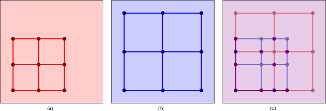
The overlay of two extended arrangements]{The overlay (c) of two arrangements (a) and (b). Each feature of the arrangements is extended with a color. The color of each feature of the overlay arrangement is the blend of the colors of the two inducing features.
The example program listed below computes the overlay, depicted in Figure 35.45, of the two arrangements depicted in (a) and (d). Each feature of the input arrangements and of the overlay arrangement is extended with an RGB color stored as an unsigned int. The vertices, halfedges, and faces of the red arrangement are assigned three different shades of red. Similarly, the vertices, halfedges, and faces of the blue arrangement are assigned three different shades of blue. Using an instance of the Overlay_color_traits class template as the overlay traits, each feature of the overlay arrangement is assigned a color that is a blend of the colors attached to the inducing features.
File Arrangement_on_surface_2/overlay_color.cpp
When you constructs an arrangement induced by a set \(\mathcal{C}\) of arbitrary two-dimensional curves, you end up with a collection \(\mathcal{C}''\) of \(x\)-monotone subcurves of \(\mathcal{C}\) that are pairwise disjoint in their interior; see Section Introduction. These subcurves are associated with the arrangement edges (more precisely, with pairs of DCEL halfedges). The connection between the originating input curves and the arrangement edges is lost during the construction process. This loss might be acceptable for some applications. However, in many practical cases it is important to determine the input curves that give rise to the final subcurves.
The Arrangement_on_surface_with_history_2<GeometryTraits,TopologyTraits> class-template extends the Arrangement_on_surface_2<GeometryTraits,TopologyTraots> class template by keeping an additional container of input curves representing \(\mathcal{C}\), and by maintaining a cross-mapping between these curves and the arrangement edges they induce. Similarly, the Arrangement_with_history_2<GeometryTraits,Dcel> class-template extends the Arrangement_2<GeometryTraits,Dcel> class template. The GeometryTraits template parameter, of either class templates, must be substituted by a model of the ArrangementTraits_2 concept; see Section Inserting General Curves. It should define the Curve_2 type and support its subdivision into X_monotone_curve_2 objects, among the others. The Dcel parameter must be substituted by a model of the ArrangementDcel concept. You can use either the default DCEL class or an extended DCEL class (see Section Extending the DCEL) based on your needs. An arrangement that support the cross-mapping mentioned above is referred to as an arrangement with history. In the following we use the Arrangement_with_history_2<> class template to demonstrate arrangements with history. However, the explanation applies also to Arrangement_on_surface_with_history_2<>, as the type of the embedding surface is irrelevant to the discussion.
The Arrangement_with_history_2 class template extends the Arrangement_2 class template. Thus, all the iterator and circulator types that are defined in the base class are also available in Arrangement_with_history_2. (Refer to Section Traversing the Arrangement for a comprehensive review of this functionality.)
As mentioned above, the Arrangement_with_history_2 class template maintains a container of input curves, which can be accessed using curve handles. Let arr identify an object, the type of which is an instance of this template. The call arr.number_of_curves() returns the number of input curves stored in the container, while arr.curves_begin() and arr.curves_end() return Arrangement_with_history_2::Curve_iterator objects that define the range of curves that induce the arrangement. The value type of this iterator is Curve_2. Moreover, the curve-iterator type is convertible to Arrangement_with_history_2::Curve_handle, which is used for accessing the stored curves. For convenience, the corresponding constant-iterator and constant-handle types are also defined.
As mentioned in the previous paragraph, a Curve_handle object ch serves as a pointer to a curve stored in an arrangement-with-history object arr. Using this handle, it is possible to obtain the number of arrangement edges this curve induces by calling arr.number_of_induced_edges(ch). The functions arr.induced_edges_begin(ch) and arr.induced_edges_end(ch) return iterators of type Arrangement_with_history_2::Induced_edges_iterator that define the range of edges induced by ch. The value type of these iterators is Halfedge_handle. It is thus possible to traverse all arrangement edges induced by an input curve.
The ability to perform the inverse mapping is also important. Given an arrangement edge, you may want to determine which input curve induces it. In case the edge represents an overlap of several curves, you should be able to trace all input curves that overlap in this edge. The Arrangement_with_history_2 class template is extended by several member functions that enable such an inverse mapping. Given a handle to halfedge e in an arrangement with history object arr, the call arr.number_of_originating_curves(e) returns the number of curves that induce the edge (which should be 1 in non-degenerate cases, and 2 or more in case of overlaps), while arr.originating_curves_begin(e) and arr.originating_curves_end(e) return Arrangement_with_history_2::Originating_curve_iterator objects that define the range of curves that induce e. The value type of these iterators is Curve_2.
Overlaying two arrangement-with-history objects is possible only if their types are instances of the Arrangement_with_history_2<Traits,Dcel> class template, where the respective Traits parameters are substituted by two traits classes that are convertible to one another. In this case, the resulting arrangement stores a consolidated container of input curves, and automatically preserves the cross-mapping between the arrangement edges and the consolidated curve-set. You may also employ an overlay-traits class to maintain any type of auxiliary data stored with the DCEL cells; see Section Overlaying Arrangements.
The Arrangement_with_history_2 class template extends the Arrangement_2 class template; thus, it inherits the fundamental modification operations, such as assign() and clear(), from it. The vertex-manipulation functions are also inherited and supported; see Sections Manipulating Isolated Vertices and Inserting Points for details. However, there are some fundamental differences between the interfaces of the two class templates, which we highlight next.
The most significant difference between the arrangement-with-history class template and the basic arrangement class template is the way they handle their input curves. Arrangement_with_history_2 always stores the Curve_2 objects that induce it. Thus, it is impossible to insert \(x\)-monotone curves into an arrangement with history. The free functions insert_non_intersecting_curve() and the version of insert() that accept \(x\)-monotone curves, as well as their aggregated versions), are therefore not available for arrangement-with-history instances. Only the free overloaded functions insert() that accept general curves, namely, the incremental insertion function and the aggregate insertion function, are supported; see Section Inserting General Curves for a review of these functions. Notice however that while the incremental insertion function insert(arr, c) for an Arrangement_2 object arr does not have a return value, the corresponding arrangement-with-history function returns a Curve_handle object that points to the inserted curve.
As we are able to keep track of all edges induced by an input curve, we also provide a free function that removes a curve from an arrangement. By calling remove_curve(arr,ch), where ch is a valid curve handle, the given curve is deleted from the curve container, and all edges induced solely by this curve (i.e., excluding overlapping edges) are removed from the arrangement. The function returns the number of edges that have been removed.
In some cases, users may need to operate directly on the arrangement edges. We first mention that the specialized insertion functions (see Section Inserting Pairwise Disjoint x-Monotone Curves) are not supported, as they accept \(x\)-monotone curves. Insertion can only be performed via the free insertion-functions. The other edge-manipulation functions (see Section Manipulating Halfedges) are, however, available, but have a different interface that does not use \(x\)-monotone curves.
Invoking split_edge(e,p) splits the edge e at a given point p that lies in its interior.
Invoking merge_edge(e1,e2) merges the two given edges. There is a precondition that e1 and e2 shared a common end-vertex of degree 2 prior to the merge, and that the \(x\)-monotone subcurves associated with these edges are mergeable.
It is possible to remove an edge by simply invoking remove_edge(e).
In all cases, the maintenance of cross-pointers for the appropriate input curves will be done automatically.
Note that it is possible to attach observers to an arrangement-with-history object in order to get detailed notifications of the changes the arrangements undergoes; see Section The Notification Mechanism for the details).
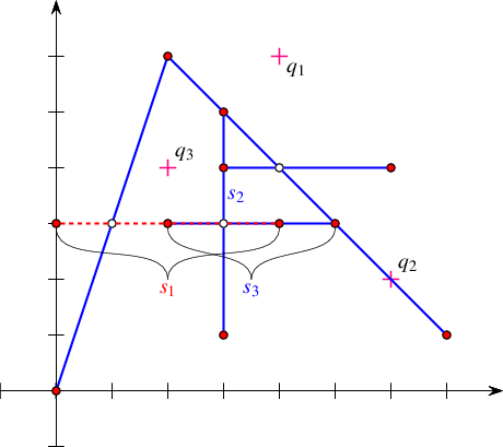
Figure 35.46 An arrangement with history as constructed in Arrangement_on_surface_2/curve_history.cpp. Note that \(s_1\) and \(s_3\) overlap over two edges. The point-location query points \(q_1\), \(q_2\), and \(q_3\) are drawn as lightly shaded dots.
In the following example we construct a simple arrangement of six line segments, as depicted in Figure 35.46, while maintaining the curve history. Note that the input segments \(s_1\) and \(s_3\) overlap over two edges. The example demonstrates the usage of the special traversal functions. It also shows how to issue point-location queries on the resulting arrangement (the query points \(q_1\), \(q_2\), and \(q_3\) are drawn as crosses), using the auxiliary function locate_point() defined in the header file point_location_utils.h; see also Section Point-Location Queries.
File Arrangement_on_surface_2/curve_history.cpp
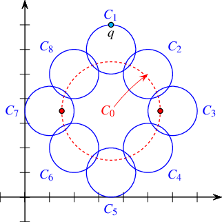
Figure 35.47 An arrangement with history of nine circles as constructed in Arrangement_on_surface_2/edge_manipulation_curve_history.cpp. Note the vertical tangency points of \(c_0\), marked as dark dots, which subdivide this circle into an upper half and a lower half, each consists of 9 edges. The large circle \(c_0\) is eventually removed from the arrangement, with all 18 edges it induces.
The following example demonstrates the usage of the free remove_curve() function. We construct an arrangement of nine circles, while keeping a handle to each inserted circle. We then remove the large circle \(c_0\), which induces \(18\) edges, as depicted in Figure 35.47. The example also shows how to use the split_edge() and merge_edge() member functions when operating on an arrangement-with-history object.
File Arrangement_on_surface_2/edge_manipulation_curve_history.cpp
In some cases, one would like to save an arrangement object constructed by some application, so that later on it can be restored. In other cases one would like to create nice drawings that represent arrangements constructed by some application. These drawings can be hard printed or displayed on a computer screen.
Consider an arrangement that represents a very complicated geographical map, and assume that there are various applications that need to answer point-location queries on this map. Naturally, you can store the set of curves that induces the arrangement, but this implies that you would need to construct the arrangement from scratch each time you need to reuse it. A more efficient solution is to write the arrangement to a file in a format that other applications can read.
This package provides an inserter (the << operator) and an extractor (the >> operator) for the Arrangement_2<Traits,Dcel> class that inserts an arrangement object into an output stream and extracts an arrangement object from an input stream, respectively. The arrangement is written using a simple predefined ASCII format that encodes the arrangement topology, as well as all geometric entities associated with vertices and edges.
The ability to use the input/output operators, requires that the Point_2 type and the X_monotone_curve_2 type defined by the traits class both support the << and >> operators. The Arr_conic_traits_2 class (see Section A Traits Class for Conic Arcs), the Arr_rational_function_traits_2 class (see Section A Traits Class for Arcs of Rational Functions), and the Arr_linear_traits_2 class (see Section Traits Classes for Line Segments and Linear Objects) currently do not provide these operators for the geometric types they define. Thus, only arrangements of line segments or of polylines can be written or read.
The following example constructs the arrangement depicted in Figure 35.7 and writes it to an output file. It also demonstrates how to re-read the arrangement from a file.
File Arrangement_on_surface_2/io.cpp
The inserter and extractor both ignore any auxiliary data stored with the arrangement features. Thus, they are ideal for arrangements instantiated using the default DCEL, which is the instance Arr_default_dcel<Traits>. However, as explained in Section Extending the DCEL, one can easily extend the arrangement faces by using the Arr_face_extended_dcel template, extend all DCEL records by using the Arr_extended_dcel template, or use the Arr_dcel template. In such cases, it might be crucial that the auxiliary data fields are written to the file and read from there.
The arrangement package includes the free functions write(arr, os, formatter), which writes the arrangement arr to an output stream os, and read(arr, os, formatter), which reads the arrangement arr from an input stream is. Both operations are performed using a formatter object, which defines the I/O format. The package contains three formatter classes:
Arr_text_formatter<Arrangement> defines a simple textual I/O format for the arrangement topology and geometry, disregarding any auxiliary data that may be associated with the arrangement features. This is the default formatter used by the arrangement inserter and the arrangement extractor, as defined above. Arr_face_extended_text_formatter<Arrangement> operates on arrangements whose DCEL representation is based on the Arr_face_extended_dcel<Traits,FaceData> class (see Section Extending the DCEL Faces). It supports reading and writing the auxiliary data objects stored with the arrangement faces provided that the FaceData class supports an inserter and an extractor. Arr_extended_dcel_text_formatter<Arrangement> operates on arrangements whose DCEL representation is based on the Arr_extended_dcel<Traits,VertexData,HalfedgeData,FaceData> class (see Section Extending All DCEL Records). It supports reading and writing the auxiliary data objects stored with the arrangement vertices, edges and faces, provided that the VertexData, HalfedgeData and FaceData classed all have inserters and extractors. The following example constructs the same arrangement as the example dcel_extension does (see Section Extending All DCEL Records), depicted in Figure 35.42, and writes it to an output file. It also demonstrates how to re-read the arrangement from a file:
File Arrangement_on_surface_2/dcel_extension_io.cpp
You may develop your own formatter classes - models of the ArrangementInputFormatter and ArrangementOutputFormatter concepts, as defined in the Reference Manual. Doing so, you can define other I/O formats, such as an XML-based format or a binary format.
Section Storing the Curve History introduces the Arrangement_with_history_2<Traits,Dcel> class, which saves the set of curves inducing an arrangement and maintains the relations between these curves and the edges they induce. Naturally, when reading or writing an arrangement-with-history instance we would like this information to be saved to the output stream or restored from the input stream alongside with the basic arrangement structure.
The arrangement package supplies an inserter and an extractor for the Arrangement_with_history_2<Traits,Dcel> class. The arrangement is represented using a simple predefined ASCII format. An object of the Arrangement_with_history_2<Traits,Dcel> type can be saved and restored, as long as the Curve_2 type defined by the traits class—as well as the Point_2 type and the X_monotone_curve_2 types—support the << and>> operators.
The following example constructs the same arrangement as example curve_history does, depicted in Figure 35.46, and writes it to an output file. It also demonstrates how to re-read the arrangement-with-history from a file:
File Arrangement_on_surface_2/io_curve_history.cpp
The arrangement package also includes the free functions write(arr,
os, formatter) and read(arr, os, formatter) that operate on a given arrangement-with-history instance arr. Both functions are parameterized by a formatter object, which defines the I/O format. The package contains a template called, Arr_with_hist_text_formatter<ArranagmentFormatter>, which extends an arrangement formatter class (see Section Arrangements with Auxiliary Data) and defines a simple textual input/output format.
An arrangement data structure can be visualized by calling the CGAL::draw<arr>() function as shown in the following example. This function opens a new window showing the given arrangement. A call to this function is blocking; that is, the program continues execution only after the user closes the window.
File Arrangement_on_surface_2/draw_arr.cpp
This function requires CGAL_Qt6, and is only available if the macro CGAL_USE_BASIC_VIEWER is defined. Linking with the cmake target CGAL::CGAL_Basic_viewer will link with CGAL_Qt6 and add the definition CGAL_USE_BASIC_VIEWER.
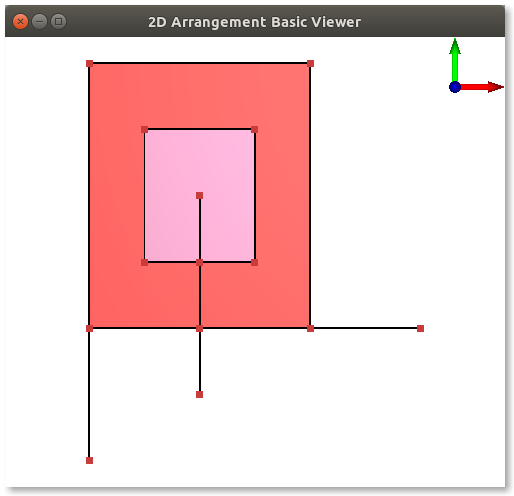
Figure 35.48 A snapshot of the window created by the program Arrangement_on_surface_2/draw_arr.cpp. The constructed arrangement consists of 14 vertices, 15 edges, and 3 faces. Notice that the colors are generated at random.
BoostSee also Boost's homepage at: www.boost.org. is a collection of portable C++ libraries that extend the C++ Standard Library. The Boost Graph Library (BGL), which one of the libraries in the collection, offers an extensive set of generic graph algorithms parameterized through templates. As our arrangements are embedded as planar graphs, it is only natural to extend the underlying data structure with the interface that the BGL expects, and gain the ability to perform the operations that the BGL supports, such as shortest-path computation. This section describes how to apply the graph algorithms implemented in the BGL to Arrangement_2 instances.
An instance of Arrangement_2 is adapted to a Boost graph through the provision of a set of free functions that operate on the arrangement features and conform with the relevant BGL concepts. Besides the straightforward adaptation, which associates a vertex with each DCEL vertex and an edge with each DCEL halfedge, the package also offer a dual adaptor, which associates a graph vertex with each DCEL face, such that two vertices are connected, iff there is a DCEL halfedge that connects the two corresponding faces.
Arrangement instances are adapted to Boost graphs by specializing the boost::graph_traits template for Arrangement_2 instances. The graph-traits states the graph concepts that the arrangement class models (see below) and defines the types required by these concepts.
In this specialization the Arrangement_2 vertices correspond to the graph vertices, where two vertices are adjacent if there is at least one halfedge connecting them. More precisely, Vertex_handle is the graph-vertex type, while Halfedge_handle is the graph-edge type. As halfedges are directed, we consider the graph to be directed as well. Moreover, as several interior-disjoint \(x\)-monotone curves (say circular arcs) may share two common endpoints, inducing an arrangement with two vertices that are connected with several edges, we allow parallel edges in our Boost.
Given an Arrangement_2 instance, we can efficiently traverse its vertices and halfedges. Thus, the arrangement graph is a model of the concepts VertexListGraph and EdgeListGraph introduced by the BGL. At the same time, we use an iterator adapter of the circulator over the halfedges incident to a vertex (Halfedge_around_vertex_circulator - see Section Traversal Methods for an Arrangement Vertex), so it is possible to go over the ingoing and outgoing edges of a vertex in linear time. Thus, our arrangement graph is a model of the concept BidirectionalGraph (this concept refines IncidenceGraph, which requires only the traversal of outgoing edges).
It is important to notice that the vertex descriptors we use are Vertex_handle Vertex_handle objects and not vertex indices. However, in order to gain more efficiency in most BGL algorithms, it is better to have them indexed \(0, 1,
\ldots, (n-1)\), where \(n\) is the number of vertices. We therefore introduce the Arr_vertex_index_map<Arrangement> class-template, which maintains a mapping of vertex handles to indices, as required by the BGL. An instance of this class must be attached to a valid arrangement vertex when it is created. It uses the notification mechanism (see Section The Notification Mechanism) to automatically maintain the mapping of vertices to indices, even when new vertices are inserted into the arrangement or existing vertices are removed.
In most algorithms provided by the BGL, the output is given by property maps, such that each map entry corresponds to a vertex. For example, when we compute the shortest paths from a given source vertex \(s\) to all other vertices we can obtain a map of distances and a map of predecessors - namely for each \(v\) vertex we have its distance from \(s\) and a descriptor of the vertex that precedes \(v\) in a shortest path from \(s\).
If the vertex descriptors are simply indices, boost supplies tools to easily represent property maps using vectors. The Arr_vertex_index_map<Arrangement> class template enables the creation of such indices, and together with boost::vector_property_map<Type, IndexMap> it generates an efficient mapping from Vertex_handle objects to properties of type Type. Note, however, that unlike the Arr_vertex_index_map class template, the vertex property-map class is not kept synchronized with the number of vertices in the arrangement, so it should not be reused in calls to BGL functions in case the arrangement is modified in between these calls.
The first example of this section demonstrates the application of Dijkstra's shortest path algorithm to compute the shortest-path length between a given vertex of an arrangement of linear curves and all other vertices. The length of a path is defined as the sum of squared Euclidean lengths of its segments. It uses an instance of the functor template Edge_length<Arrangement>} to compute the squared Euclidean length of the linear curve associated with a given halfedge of the arrangement. The functor implements a Boost property-map that attaches square lengths to edges; when the BGL algorithm queries the property map for a squared length of an edge the property map computes and returns it. The functor template is defined in the header file Edge_length.h.
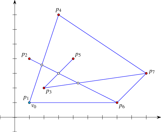
Figure 35.49 An arrangement of seven line segments, as constructed by Arrangement_on_surface_2/bgl_primal_adapter.cpp and Arrangement_on_surface_2/bgl_dual_adapter.cpp.
In the following example we construct an arrangement of seven line segments, as shown in Figure 35.49. Then, it uses the BGL generic implementation of Dijkstra's shortest-paths algorithm to compute the sum of squared distances to all vertices from the lexicographically smallest vertex \(v_0\) in the arrangement. Note the usage of the Arr_vertex_property_map class template in the call to boost::dijkstra_shortest_paths() and in the definition of the distance property-map. We instantiate a property map that attaches a number of type Number_type (which is a type of unlimited precision) to each vertex. The number represents the sum of squared distances of the vertex from \(v_0\).
File Arrangement_on_surface_2/bgl_primal_adapter.cpp
An arrangement instance can be represented as a graph other than the one described in the previous section. A dual-graph representation refers to the graph, where each arrangement face corresponds to a graph vertex, and two vertices are adjacent iff the corresponding faces share a common edge on their boundaries. This is done by specializing the boost::graph_traits template for Dual<Arrangement_2> instances, where Dual<Arrangement_2> is a template specialization that gives a dual interpretation to an arrangement instance.
In a dual representation, Face_handle is the graph-vertex type, while Halfedge_handle is the graph-edge type. We treat the graph edges as directed, such that a halfedge e is directed from \(f_1\), which is its incident face, to \(f_2\), which is the incident face of its twin halfedge. As two arrangement faces may share more than a single edge on their boundary, we allow parallel edges (loops) in our Boost graph. As is the case in the primal graph, the dual arrangement graph is also a model of the concepts VertexListGraph, EdgeListGraph and BidirectionalGraph (thus also of IncidenceGraph).
Since we use Face_handle objects as the vertex descriptors, we define the Arr_face_index_map<Arrangement> class-template, which maintains an efficient mapping of face handles to indices.
The next example demonstrates how a property map can be used to update or receive information directly from a feature of the arrangement without the need to search for its index. The example also demonstrates the application of the breadth-first search} (BFS) algorithm on a dual arrangement. It uses the functor template Extended_face_property_map<Arrangement, Type> to directly access information stored inside the faces. The functor implements a property map that utilizes the data() and set_data() member functions of the extended face to update or obtain the property. When the property map is instantiated, the Type parameter must be substituted by the same type that is used to extend the arrangement face; see Section Extending the DCEL Faces. The functor template is defined in the header file Extended_face_property_map.h listed below.
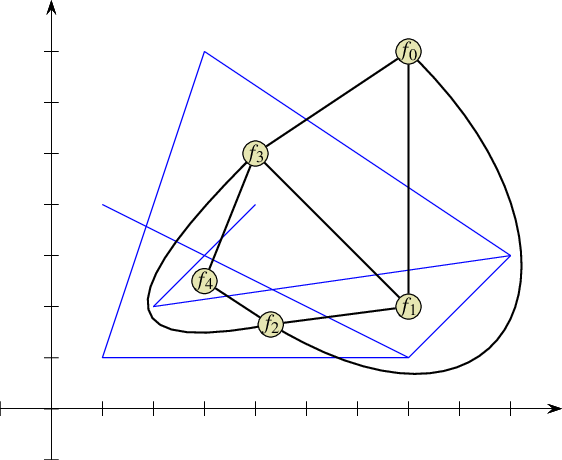
Figure 35.50 An arrangement of seven line segments, as constructed by Arrangement_on_surface_2/bgl_dual_adapter.cpp and its dual face graph, where every arrangement face is a vertex of the graph. The index of a dual vertex is the discovery time of a breadth-first search applied to the face graph, starting from the unbounded face \(f_0\).
The following example constructs the same arrangement constructed by the program coded in Arrangement_on_surface_2/bgl_primal_adapter.cpp; see Figure 35.49. Then, it performs a breadth-first search traversal on the face graph, starting from the unbounded face. The DCEL faces are extended with an unsigned integer indicating the discovered time of the face. The code uses a visitor that obtains the times and writes them into a property map that updates the faces accordingly. Figure 35.50 shows the graph dual to the arrangement. It is clear that the unbounded face \(f_0\) is discovered at time \(0\), the neighboring faces \(f_1\), \(f_3\), and \(f_4\) are discovered at times \(1\), \(2\), and \(3\), and finally \(f_2\) is discovered at time \(4\).
File Arrangement_on_surface_2/bgl_dual_adapter.cpp
Before the specific tips, we remind you that compiling programs with debug flags disabled and with optimization flags enabled significantly reduces the running time.
When the curves to be inserted into an arrangement are \(x\)-monotone and pairwise disjoint in their interior to start with, then it is more efficient (in running time) and less demanding (in traits-class functionality) to use the non-intersecting insertion-functions instead of the general ones; e.g., insert().
When the curves to be inserted into an arrangement are segments that are pairwise disjoint in their interior, it is more efficient to use the traits class Arr_non_caching_segment_traits_2 rather than the default one (Arr_segment_traits_2).
If the segments may intersect each other, the default traits class Arr_segment_traits_2 can be safely used with the somehow limited number type Quotient<MP_float>.
On rare occasions the traits class Arr_non_caching_segment_traits_2 exhibits slightly better performance than the default one (Arr_segment_traits_2 even when the segments intersect each other, due to the small overhead of the latter (optimized) traits class. (For example, when the so-called LEDA rational kernel is used.)
Prior knowledge of the combinatorial structure of the arrangement can be used to accelerate operations that insert \(x\)-monotone curves, whose interior is disjoint from existing edges and vertices of the arrangement. The specialized insertion functions, i.e., Arrangement_on_surface_2::insert_in_face_interior(), Arrangement_on_surface_2::insert_from_left_vertex(), Arrangement_on_surface_2::insert_from_right_vertex(), and Arrangement_on_surface_2::insert_at_vertices() can be used according to the available information. These functions hardly involve any geometric operations, if at all. They accept topologically related parameters, and use them to operate directly on the DCEL records, thus saving algebraic operations, which are especially expensive when high-degree curves are involved.
A polygon, represented by a list of segments along its boundary, can be inserted into an empty arrangement as follows. First, one segment is inserted using Arrangement_on_surface_2::insert_in_face_interior() into the unbounded face. Then, a segment with a common end point is inserted using either Arrangement_on_surface_2::insert_from_left_vertex() or Arrangement_on_surface_2::insert_from_right_vertex(), and so on with the rest of the segments except for the last, which is inserted using Arrangement_on_surface_2::insert_at_vertices(), as both endpoints of which are the mapping of known vertices.
The main trade-off among point-location strategies is between time and storage. Using the naive or walk strategies, for example, takes more query time but does not require preprocessing or maintenance of auxiliary structures and saves storage space.
If point-location queries are not performed frequently, but other modifying functions, such as removing, splitting, or merging edges are, then using a point-location strategy that does not require the maintenance of auxiliary structures, such as the naive or walk strategies, is preferable.
There is a trade-off between two modes of the trapezoidal RIC strategy that enables the user to choose whether preprocessing should be performed or not. If preprocessing is not used, the creation of the structure is faster. However, for some input sequences the structure might be unbalanced and therefore queries and updates might take longer, especially, if many removal and split operations are performed.
When the curves to be inserted into an arrangement are available in advance (as opposed to supplied on-line), it is advised to use the more efficient aggregate (sweep-based) insertion over the incremental insertion; e.g., insert(arr, first, last).
The various traits classes should be instantiated with an exact number type to ensure robustness when the input of the operations to be carried out might be degenerate. Inexact number types can be used at the user's own risk.
Maintaining short bit-lengths of coordinate representations may drastically decrease the time consumption of arithmetic operations on the coordinates. This can be achieved by caching certain information or normalization (of rational numbers). However, both solutions should be used cautiously, as the former may lead to an undue space consumption, and indiscriminate normalization may considerably slow down the overall process.
The code of this package is the result of a long development process. Initially (and until version 3.1), the code was spread among several components, namely, Topological_map, Planar_map_2, Planar_map_with_intersections_2 and Arrangement_2, that were developed by Ester Ezra, Eyal Flato, Efi Fogel, Dan Halperin, Iddo Hanniel, Idit Haran, Shai Hirsch, Eugene Lipovetsky, Oren Nechushtan, Sigal Raab, Ron Wein, Baruch Zukerman, and Tali Zvi.
In version 3.2, as part of the ACS project, the packages have gone through a major re-design, resulting in an improved and unified 2D Arrangements package. The code of the new package was restructured and developed by Efi Fogel, Idit Haran, Ron Wein, and Baruch Zukerman. This version included for the first time a new geometry-traits class that handles circular and linear curves, and is based on the circular kernel. The circular kernel was developed by Monique Teillaud, Sylvain Pion, and Julien Hazebrouck.
Version 3.3 features arrangements of unbounded curves for the first time. The design and development of this feature required yet another restructuring of the entire package. All this was done by Eric Berberich, Efi Fogel, Dan Halperin, Ophir Setter, and Ron Wein. Michael Hemmer helped tuning up parts of the geometry-traits concept related to unbounded curves.
Version 3.7 introduced a geometry-traits class that handles planar algebraic curves of arbitrary degree. It was developed by Eric Berberich and Michael Kerber.
Version 3.9 introduced a new geometry-traits class that handles rational arcs. It was developed by Oren Salzman and Michael Hemmer. It replaced an old traits, which handled the same family of curves, developed by Ron Wein.
Version 4.1 introduces a revised implementation of the point location class via a randomized incremental construction of the trapezoidal map. The old class was implemented by Oren Nechushtan, while the revamp was done by Michal Kleinbort and Michael Hemmer. The new class adds support for unbounded curves and can now guarantee logarithmic query time in all cases.