User Manual

Author

Amal Dev Parakkat, Stefan Ohrhallinger, Elmar Eisemann, Pooran Memari

This CGAL component implements a surface reconstruction method that takes an unoriented set of 3D points as input and computes a piecewise linear approximation of the sampled surface. In simple words, the method tries to classify the medial balls (computed from the 3D Delaunay triangulation of the input points) into interior and exterior and returns the interface between them.

The detailed description of the algorithm can be seen in [2].

Definitions

The method is built upon the fact that whenever a discrete set of sample points approximates a continuous surface, the Voronoi balls (interior/exterior) intersect along the boundary with a ratio inversely proportional to the sampling density (similar to the observation of Amenta et al. [1]). Based on this, we define an intersection ratio between adjacent Voronoi balls as follows:

\( ir(B_0,B_1) = max((r_0+r_1-d)/r_0,(r_0+r_1-d)/r_1) \)

Where \( B_0 \) and \( B_1 \) are two adjacent Voronoi balls with radius \( r_0 \) and \( r_1 \) respectively, and \( d \) is the distance between it's circumcenters.

Using this ratio, we can say that if the intersection ratio between two adjacent Voronoi balls is small, they likely correspond to a pair of interior and exterior balls sharing a thin overlapping region along the underlying surface (a 2D case is illustrated in Figure Figure 71.1). In other words, given a threshold \( \delta \), a triangle is said to belong to a set \( BallMerge(\delta) \) if its corresponding adjacent Voronoi balls have an intersection ratio less than \( \delta \). By definition, \( BallMerge(\delta) \) is a subcomplex of the Delaunay triangulation of the sample points. It is easy to see that \( BallMerge(0) \) is empty, while \( BallMerge(\delta) \), for any \( \delta \gt 2 \) contains all the triangles of the Delaunay triangulation.

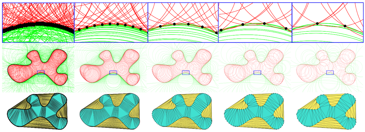
Figure 71.1 Top: The interior (red) and exterior (green) medial balls of a point set with decreasing point density from l.t.r. Bottom: Corresponding \( \delta \)-merged components on Delaunay triangulation.

CGAL provides the global variant of BallMerge as described in [2].

ball_merge_surface_reconstruction(): Given a threshold \( \delta \), two Delaunay simplices are called \( \delta\)-merged either if their corresponding Voronoi balls are adjacent with an intersection ratio \( > \delta \) or if there exists another Delaunay simplex, which is \( \delta\)-merged with both of them. Following a procedure similar to classical connected component computation, the algorithm starts by visiting \( \delta\)-merged simplices from an arbitrary seed simplex (the procedure is order independent) and tag them with the current component label until no more \( \delta\)-merged simplices remain. The procedure is then restarted with any yet unvisited simplex until all have been visited, and output the simplices with the most frequent label. The reconstructed surface is then computed from the boundary of this output.

Input Requirements

This method expects as input a 3D point cloud sampled a manifold close surface with a single connected component. It always returns a watertight and manifold surface triangle mesh. As the algorithm attempts to close the surface, it can tolerate some missing data and can handle little outliers and noise. If there are some significant gaps in the data, the internal flooding algorithm will generate triangle faces from points visible from inside the input surface.

Parameter Settings

The main parameter used in \( BallMerge \) is the intersection ratio \(\delta\). By definition, \(\delta\) ranges from 0 to 2, with \( BallMerge(0) \) being empty and \( BallMerge(2) \) containing all the triangles of the Delaunay triangulation. Experiments show that the \( > \delta \) value usually lies between 1.5 and 1.95, with 1.8 or 1.85 yielding the best results in most cases. Thanks to the useful properties of this intersection ratio, tuning this parameter can be done using the following rule: if the reconstructed surface has missing parts, the threshold should be lowered, conversely, if the reconstructed surface has additional parts, the threshold should be increased.

If no value is provided to the reconstruction function, the \(\delta\) parameter is automatically estimated using the following method: Starting from the maximal value 2, we iteratively decrease \(\delta\) until the reconstructed surface undergoes a sudden vertex-count drop (10% of the total number of input points). This indicates that a large number of interior/exterior medial balls have become \(\delta\)-merged, causing that part of the reconstructed surface to collapse. Consequently, the value from the previous iteration is used to generate the output. The \(\delta\) value used is always returned by the functions.

Examples

ball_merge_surface_reconstruction() has the following arguments: The set of input points, two output parameters where the resulting meshes will be stored, and optionally the parameter \( \delta \). The function returns two meshes - the largest and second-largest components as sometimes the expected shape will be the second-largest component after merging. A sample program showing how to use this function is given below, together with the output reconstructions.

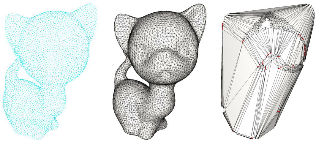
Figure 71.2 Results of the run of the ball merge algorithm with automatic delta parameter estimation. From left to right: Input point cloud (no normal required); one of the two output containing the expected triangle mesh; the second output representing the non desired part, that is actually a triangle soup with non-manifold edges (shown in red). The delta parameter that is automatically estimated is 1.

File Ball_merge_surface_reconstruction/ball_merge_reconstruction.cpp

#include <CGAL/Exact_predicates_inexact_constructions_kernel.h>
#include <CGAL/Ball_merge_surface_reconstruction.h>
#include <CGAL/IO/polygon_soup_io.h>
#include <CGAL/IO/read_points.h>
 
#include <string>
 
typedef CGAL::Exact_predicates_inexact_constructions_kernel K;
typedef K::Point_3 Point;
 
namespace params=CGAL::parameters;
 
int main(int argc, char **argv)
{
  // reading input points and parameters
  const std::string inFilename=argc>1?argv[1]:CGAL::data_file_path("points_3/kitten.xyz");
 
  std::vector<Point> points;
  CGAL::IO::read_points(inFilename, std::back_inserter(points));
 
  if (points.empty())
  {
    std::cerr << inFilename << " cannot be read correctly or is empty.\n";
    return 1;
  }
 
  //vectors for storing output triangle indices
  std::vector<std::array<int,3>> meshFaceIndices1, meshFaceIndices2;
 
  double delta = argc > 2
    // run the reconstruction with user passed delta parameter
    ? CGAL::ball_merge_surface_reconstruction(points,
                                              meshFaceIndices1, meshFaceIndices2,
                                              params::delta(atof(argv[2]))
                                                     .concurrency_tag(CGAL::Parallel_if_available_tag()))
 
  // run the reconstruction with automatic parameter estimation
    : CGAL::ball_merge_surface_reconstruction(points,
                                              meshFaceIndices1, meshFaceIndices2,
                                              params::concurrency_tag(CGAL::Parallel_if_available_tag()));
 
  // write output triangle soups
  CGAL::IO::write_polygon_soup("BMOut1.ply", points, meshFaceIndices1); //The first resulting mesh
  CGAL::IO::write_polygon_soup("BMOut2.ply", points, meshFaceIndices2); //The second resulting mesh
 
  std::cout << "delta parameter used = " << delta << "\n";
 
  return 0;
}

Ideally, the current implementation takes a dense point cloud as input (plain x,y,z coordinates without any additional information like normal or texture) sampled over a smooth surface. Thanks to the "intersection ratio", the algorithm can also handle a few challenging cases with mild noise, outliers or missing data up to an extent. It is worth noting that outliers sometimes create deep cavities over the surface, and an increased amount of noise shrinks and sometimes misses important features.

Finally, the algorithm is efficient, requiring minimal computation resources relative to the input size, as it completes two swift linear-time passes over the 3D Delaunay triangulation.

Implementation History

This package is based on the original code from the research article [2] and has been turned into a CGAL package by Amel Dev Parakkat and Sébastien Loriot.