- Author
- Simon Giraudot
Many sensors used in GIS applications (for example LIDAR), generate dense point clouds. Such applications often take advantage of more advanced data structures: for example, Triangulated Irregular Networks (TIN) that can be the base for Digital Evelation Models (DEM) and in particular for the generation of Digital Terrain Models (DTM). Point clouds can also be enriched by classification information that segments the points into ground, vegetation and building points (or other user-defined labels).
The definitions of some data structures may vary according to different sources. We will use the following terms within this tutorial:
- TIN: Triangulated Irregular Network, a 2D triangulation structure that connects 3D points based on their projections on the horizontal plane.
- DSM: Digital Surface Model, a model of the whole scanned surface including buildings and vegetation. We use a TIN to store the DSM.
- DTM: Digital Terrain Model, a model of the bare ground surface without objects like buildings or vegetation. We both use a TIN and a raster to store a DTM.
- DEM: Digital Elevation Model, a more general term that includes both DSM and DTM.
This tutorial illustrates the following scenario. From an input point cloud, we first compute a DSM stored as a TIN. Then, we filter out overly large facets that correspond either to building facades or to vegetation noise. Large components corresponding to the ground are kept. Holes are filled and the obtained DEM is remeshed. A raster DEM and a set of contour polylines are generated from it. Finally, supervised 3-label classification is performed to segment vegetation, building and group points.
Triangulated Irregular Network (TIN)
CGAL provides several triangulation data structures and algorithms. A TIN can be generated by combining the 2D Delaunay triangulation with projection traits: the triangulation structure is computed using the 2D positions of the points along a selected plane (usually, the XY-plane), while the 3D positions of the points are kept for visualization and measurements.
A TIN data structure can thus simply be defined the following way:
Digital Surface Model (DSM)
Point clouds in many formats (XYZ, OFF, PLY, LAS) can be easily loaded into a CGAL::Point_set_3 structure, using the stream operator. Generating a DSM stored in TIN is then straightforward:
std::ifstream ifile (fname, std::ios_base::binary);
ifile >> points;
std::cerr << points.size() << " point(s) read" << std::endl;
TIN dsm (points.points().begin(), points.points().end());
Because the Delaunay triangulation of CGAL is a model of FaceGraph, it is straightforward to convert the generated TIN into a mesh structure such as CGAL::Surface_mesh and be saved into whatever formats are supported by such structure:
Mesh dsm_mesh;
std::ofstream dsm_ofile ("dsm.ply", std::ios_base::binary);
dsm_ofile.close();
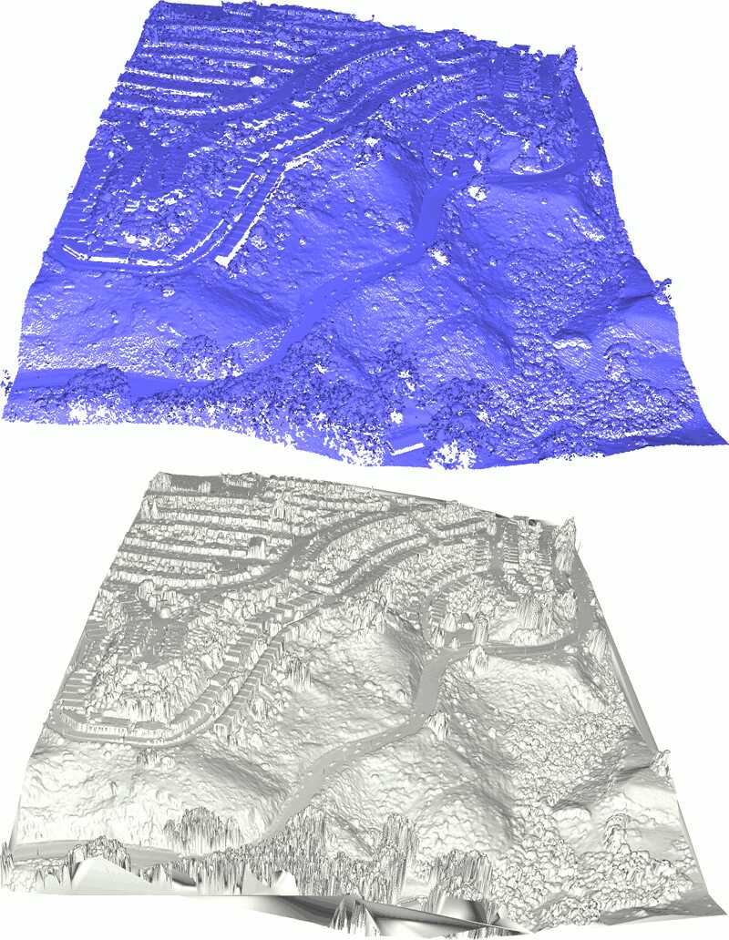
An example of a DSM computed this way on the San Fransisco data set (see References) is given in Figure 0.1.
Digital Terrain Model (DTM)
The generated DSM is used as a base for DTM computation, that is a representation of the ground as another TIN after filtering non-ground points.
We propose, as an example, a simple DTM estimation decomposed in the following steps:
- Thresholding the height of the facets to remove brutal changes of elevation
- Clustering the other facets into connected components
- Filtering all components smaller than a user-defined threshold
This algorithm relies on 2 parameters: a height threshold that corresponds to the minimum height of a building, and a perimeter threshold that corresponds to the maximum size of a building on the 2D projection.
TIN With Info
Because it takes advantage of the flexible CGAL Delaunay triangulation API, our TIN can be enriched with information on vertices and/or on faces. In our case, each vertex keeps track of the index of the corresponding point in the input point cloud (which will allow to filter ground points afterwards), and each face is given the index of its connected component.
auto idx_to_point_with_info
= [&](const Point_set::Index& idx) -> std::pair<Point_3, Point_set::Index>
{
return std::make_pair (points.point(idx), idx);
};
TIN_with_info tin_with_info
(boost::make_transform_iterator (points.begin(), idx_to_point_with_info),
boost::make_transform_iterator (points.end(), idx_to_point_with_info));
Identifying Connected Components
Connected components are identified through a flooding algorithm: from a seed face, all incident faces are inserted in the current connected component unless their heights exceed the user-defined threshold.
double spacing = CGAL::compute_average_spacing<Concurrency_tag>(points, 6);
spacing *= 2;
auto face_height
= [&](const TIN_with_info::Face_handle fh) -> double
{
double out = 0.;
for (int i = 0; i < 3; ++ i)
out = (
std::max) (out,
CGAL::abs(fh->vertex(i)->point().z() - fh->vertex((i+1)%3)->point().z()));
return out;
};
for (TIN_with_info::Face_handle fh : tin_with_info.all_face_handles())
if (tin_with_info.is_infinite(fh) || face_height(fh) > spacing)
fh->info() = -2;
else
fh->info() = -1;
std::vector<int> component_size;
for (TIN_with_info::Face_handle fh : tin_with_info.finite_face_handles())
{
if (fh->info() != -1)
continue;
std::queue<TIN_with_info::Face_handle> todo;
todo.push(fh);
int size = 0;
while (!todo.empty())
{
TIN_with_info::Face_handle current = todo.front();
todo.pop();
if (current->info() != -1)
continue;
current->info() = int(component_size.size());
++ size;
for (int i = 0; i < 3; ++ i)
todo.push (current->neighbor(i));
}
component_size.push_back (size);
}
std::cerr << component_size.size() << " connected component(s) found" << std::endl;
This TIN enriched with connected component information can be saved as a colored mesh:
Mesh tin_colored_mesh;
Mesh::Property_map<Mesh::Face_index, CGAL::IO::Color>
color_map = tin_colored_mesh.add_property_map<Mesh::Face_index,
CGAL::IO::Color>(
"f:color").first;
CGAL::parameters::face_to_face_output_iterator
(boost::make_function_output_iterator
([&](const std::pair<TIN_with_info::Face_handle, Mesh::Face_index>& ff)
{
if (ff.first->info() < 0)
else
{
r.get_int(64, 192),
r.get_int(64, 192));
}
})));
std::ofstream tin_colored_ofile ("colored_tin.ply", std::ios_base::binary);
tin_colored_ofile.close();
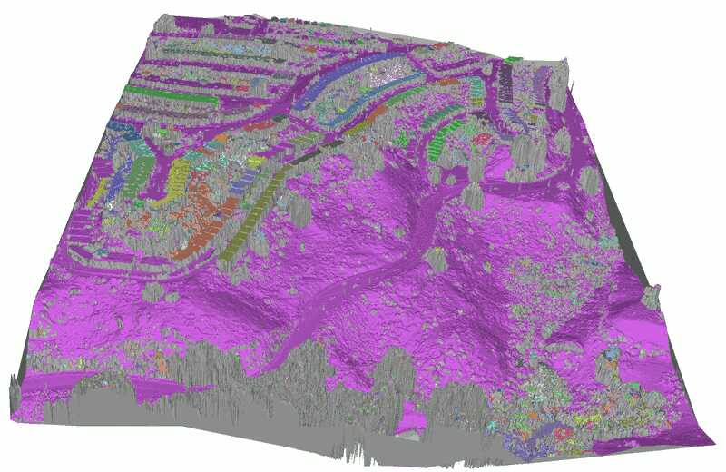
An example of a TIN colored by connected components is given in Figure 0.2.
Filtering
Components smaller than the largest building can be removed this way:
int min_size = int(points.size() / 2);
std::vector<TIN_with_info::Vertex_handle> to_remove;
for (TIN_with_info::Vertex_handle vh : tin_with_info.finite_vertex_handles())
{
TIN_with_info::Face_circulator circ = tin_with_info.incident_faces (vh),
start = circ;
bool keep = false;
do
{
if (circ->info() >= 0 && component_size[std::size_t(circ->info())] > min_size)
{
keep = true;
break;
}
}
while (++ circ != start);
if (!keep)
to_remove.push_back (vh);
}
std::cerr << to_remove.size() << " vertices(s) will be removed after filtering" << std::endl;
for (TIN_with_info::Vertex_handle vh : to_remove)
tin_with_info.remove (vh);
Hole Filling and Remeshing
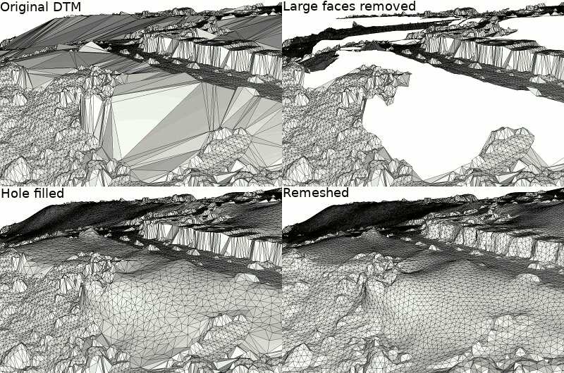
Because simply removing vertices in the large areas covered by buildings results in large Delaunay faces that offer a poor 3D representation of the DTM, an additional step can help producing better shaped meshes: faces larger than a threshold are removed and filled with a hole filling algorithm that triangulates, refines and fairs the holes.
The following snippet copies the TIN into a mesh while filtering out overly large faces, then identifies the holes and fills them all except for the largest one (which is the outer hull).
Mesh dtm_mesh;
std::vector<Mesh::Face_index> face_selection;
Mesh::Property_map<Mesh::Face_index, bool> face_selection_map
= dtm_mesh.add_property_map<Mesh::Face_index, bool>("is_selected", false).first;
CGAL::parameters::face_to_face_output_iterator
(boost::make_function_output_iterator
([&](const std::pair<TIN_with_info::Face_handle, Mesh::Face_index>& ff)
{
double longest_edge = 0.;
bool border = false;
for (int i = 0; i < 3; ++ i)
{
(ff.first->vertex((i+1)%3)->point(),
ff.first->vertex((i+2)%3)->point()));
TIN_with_info::Face_circulator circ
= tin_with_info.incident_faces (ff.first->vertex(i)),
start = circ;
do
{
if (tin_with_info.is_infinite (circ))
{
border = true;
break;
}
}
while (++ circ != start);
if (border)
break;
}
if (!border && longest_edge > limit)
{
face_selection_map[ff.second] = true;
face_selection.push_back (ff.second);
}
})));
std::ofstream dtm_ofile ("dtm.ply", std::ios_base::binary);
dtm_ofile.close();
std::cerr << face_selection.size() << " face(s) are selected for removal" << std::endl;
face_selection.clear();
for (Mesh::Face_index fi : faces(dtm_mesh))
if (face_selection_map[fi])
face_selection.push_back(fi);
std::cerr << face_selection.size() << " face(s) are selected for removal after expansion" << std::endl;
for (Mesh::Face_index fi : face_selection)
dtm_mesh.collect_garbage();
if (!dtm_mesh.is_valid())
std::cerr << "Invalid mesh!" << std::endl;
std::ofstream dtm_holes_ofile ("dtm_with_holes.ply", std::ios_base::binary);
dtm_holes_ofile.close();
std::vector<Mesh::Halfedge_index> holes;
std::cerr << holes.size() << " hole(s) identified" << std::endl;
double max_size = 0.;
Mesh::Halfedge_index outer_hull;
for (Mesh::Halfedge_index hi : holes)
{
{
const Point_3& p = dtm_mesh.point(target(haf, dtm_mesh));
hole_bbox += p.bbox();
}
Point_2(hole_bbox.
xmax(), hole_bbox.
ymax()));
if (size > max_size)
{
max_size = size;
outer_hull = hi;
}
}
for (Mesh::Halfedge_index hi : holes)
if (hi != outer_hull)
std::ofstream dtm_filled_ofile ("dtm_filled.ply", std::ios_base::binary);
dtm_filled_ofile.close();
Isotropic remeshing can also be performed as a final step in order to produce a more regular mesh that is not constrained by the shape of 2D Delaunay faces.
std::ofstream dtm_remeshed_ofile ("dtm_remeshed.ply", std::ios_base::binary);
dtm_remeshed_ofile.close();
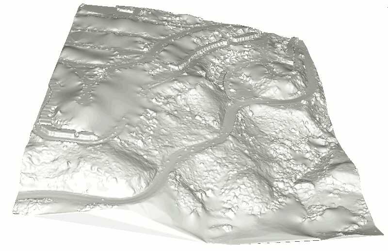
Figure 0.3 shows how these different steps affect the output mesh and Figure 0.4 shows the DTM isotropic mesh.
Rastering
The TIN data structure can be combined with barycentric coordinates in order to interpolate and thus rasterize a height map at any resolution needed the information embedded in the vertices.
Because the latest two steps (hole filling and remeshing) were performed on a 3D mesh, the hypothesis that our DTM is a 2.5D representation may no longer be valid. We thus first rebuild a TIN using the vertices of the isotropic DTM mesh lastly computed.
The following snippet generates a raster image of the height in the form of rainbow ramp PPM file (simple bitmap format):
CGAL::Bbox_3 bbox = CGAL::bbox_3 (points.points().begin(), points.points().end());
std::size_t width = 1920;
std::size_t height = std::size_t((bbox.
ymax() - bbox.
ymin()) * 1920 / (bbox.
xmax() - bbox.
xmin()));
std::cerr << "Rastering with resolution " << width << "x" << height << std::endl;
std::ofstream raster_ofile ("raster.ppm", std::ios_base::binary);
raster_ofile << "P6" << std::endl
<< width << " " << height << std::endl
<< 255 << std::endl;
Color_ramp color_ramp;
TIN::Face_handle location;
for (std::size_t y = 0; y < height; ++ y)
for (std::size_t x = 0; x < width; ++ x)
{
Point_3 query (bbox.
xmin() + x * (bbox.
xmax() - bbox.
xmin()) /
double(width),
bbox.
ymin() + (height-y) * (bbox.
ymax() - bbox.
ymin()) /
double(height),
0);
location = dtm_clean.locate (query, location);
std::array<unsigned char, 3> colors { 0, 0, 0 };
if (!dtm_clean.is_infinite(location))
{
(Point_2 (location->vertex(0)->point().x(), location->vertex(0)->point().y()),
Point_2 (location->vertex(1)->point().x(), location->vertex(1)->point().y()),
Point_2 (location->vertex(2)->point().x(), location->vertex(2)->point().y()),
Point_2 (query.x(), query.y()),
Kernel());
double height_at_query
= (barycentric_coordinates[0] * location->vertex(0)->point().z()
+ barycentric_coordinates[1] * location->vertex(1)->point().z()
+ barycentric_coordinates[2] * location->vertex(2)->point().z());
double height_ratio = (height_at_query - bbox.
zmin()) / (bbox.
zmax() - bbox.
zmin());
colors = color_ramp.get(height_ratio);
}
raster_ofile.write (reinterpret_cast<char*>(&colors), 3);
}
raster_ofile.close();
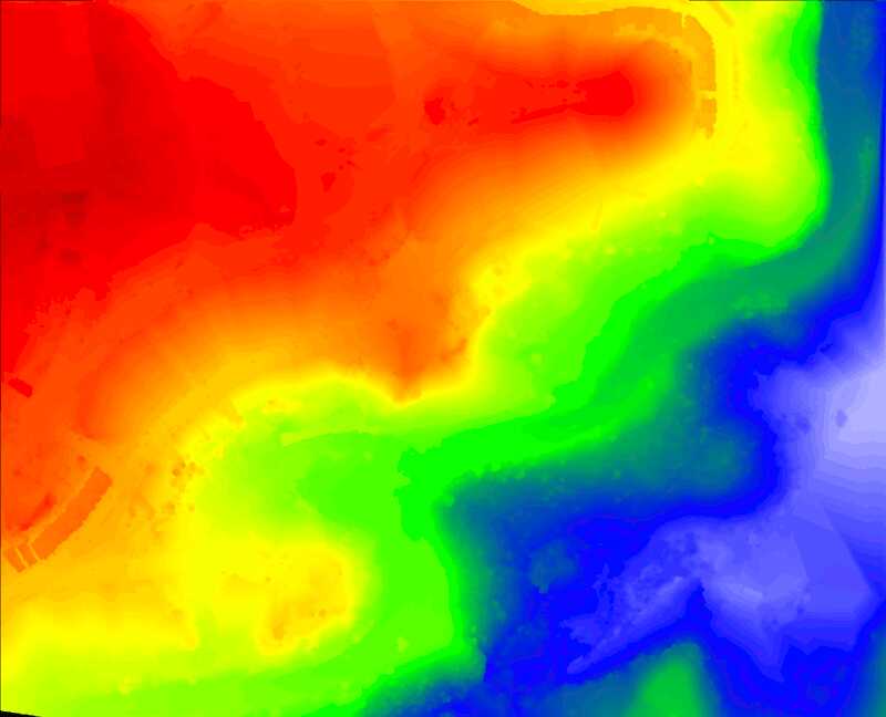
An example of a raster image with a rainbow ramp representing height is given in Figure 0.5.
Contouring
Extracting isolevels of a function defined on a TIN is another application that can be done with CGAL. We demonstrate here how to extract isolevels of height to build a topographic map.
Building a Contour Graph
The first step is to extract, from all faces of the triangulation, the section of each isolevel that goes through that face, in the form of a segment. The following functions allow to test if one isovalue does cross a face, and to extract it then:
bool face_has_isovalue (TIN::Face_handle fh, double isovalue)
{
bool above = false, below = false;
for (int i = 0; i < 3; ++ i)
{
if (fh->vertex(i)->point().z() > isovalue)
above = true;
if (fh->vertex(i)->point().z() < isovalue)
below = true;
}
return (above && below);
}
Segment_3 isocontour_in_face (TIN::Face_handle fh, double isovalue)
{
Point_3 source;
Point_3 target;
bool source_found = false;
for (int i = 0; i < 3; ++ i)
{
Point_3 p0 = fh->vertex((i+1) % 3)->point();
Point_3 p1 = fh->vertex((i+2) % 3)->point();
if ((p0.z() - isovalue) * (p1.z() - isovalue) > 0)
continue;
double zbottom = p0.z();
double ztop = p1.z();
if (zbottom > ztop)
{
}
double ratio = (isovalue - zbottom) / (ztop - zbottom);
if (source_found)
target = p;
else
{
source = p;
source_found = true;
}
}
return Segment_3 (source, target);
}
From these functions, we can create a graph of segments to process later into a set of polylines. To do so, we use the boost::adjacency_list structure and keep track of a mapping from the positions of the end points to the vertices of the graph.
The following code computes 50 isovalues evenly distributed between the minimum and maximum heights of the point cloud and creates a graph containing all isolevels:
std::array<double, 50> isovalues;
for (std::size_t i = 0; i < isovalues.size(); ++ i)
isovalues[i] = bbox.
zmin() + ((i+1) * (bbox.
zmax() - bbox.
zmin()) / (isovalues.size() - 2));
using Segment_graph = boost::adjacency_list<boost::listS, boost::vecS, boost::undirectedS, Point_3>;
Segment_graph graph;
using Map_p2v = std::map<Point_3, Segment_graph::vertex_descriptor>;
Map_p2v map_p2v;
for (TIN::Face_handle vh : dtm_clean.finite_face_handles())
for (double iv : isovalues)
if (face_has_isovalue (vh, iv))
{
Segment_3 segment = isocontour_in_face (vh, iv);
for (const Point_3& p : { segment.source(), segment.target() })
{
Map_p2v::iterator iter;
bool inserted;
std::tie (iter, inserted) = map_p2v.insert (std::make_pair (p, Segment_graph::vertex_descriptor()));
if (inserted)
{
iter->second = boost::add_vertex (graph);
graph[iter->second] = p;
}
}
boost::add_edge (map_p2v[segment.source()], map_p2v[segment.target()], graph);
}
Splitting Into Polylines
Once the graph is created, splitting it into polylines is easily performed using the function CGAL::split_graph_into_polylines() :
std::vector<std::vector<Point_3> > polylines;
Polylines_visitor<Segment_graph> visitor (graph, polylines);
std::cerr << polylines.size() << " polylines computed, with "
<< map_p2v.size() << " vertices in total" << std::endl;
std::ofstream contour_ofile ("contour.wkt");
contour_ofile.precision(18);
contour_ofile.close();
This function requires a visitor which is called when starting a polyline, when adding a point to it and when ending it. Defining such a class is straightforward in our case:
template <typename Graph>
class Polylines_visitor
{
private:
std::vector<std::vector<Point_3> >& polylines;
Graph& graph;
public:
Polylines_visitor (Graph& graph, std::vector<std::vector<Point_3> >& polylines)
: polylines (polylines), graph(graph) { }
void start_new_polyline()
{
polylines.push_back (std::vector<Point_3>());
}
void add_node (typename Graph::vertex_descriptor vd)
{
polylines.back().push_back (graph[vd]);
}
void end_polyline()
{
if (polylines.back().size() < 50)
polylines.pop_back();
}
};
Simplifying
Because the output is quite noisy, users may want to simplify the polylines. CGAL provides a polyline simplification algorithm that guarantees that two polylines won't intersect after simplification. This algorithm takes advantage of the CGAL::Constrained_triangulation_plus_2, which embeds polylines as a set of constraints:
using CDT_vertex_base = PS::Vertex_base_2<Projection_traits>;
The following code simplifies the polyline set based on the squared distance to the original polylines, stopping when no more vertex can be removed without going farther than 4 times the average spacing.
CTP ctp;
for (const std::vector<Point_3>& poly : polylines)
ctp.insert_constraint (poly.begin(), poly.end());
PS::simplify (ctp, PS::Squared_distance_cost(), PS::Stop_above_cost_threshold (16 * spacing * spacing));
polylines.clear();
for (CTP::Constraint_id cid : ctp.constraints())
{
polylines.push_back (std::vector<Point_3>());
polylines.back().reserve (ctp.vertices_in_constraint (cid).size());
for (CTP::Vertex_handle vh : ctp.vertices_in_constraint(cid))
polylines.back().push_back (vh->point());
}
std::size_t nb_vertices
= std::accumulate (polylines.begin(), polylines.end(), std::size_t(0),
[](std::size_t size, const std::vector<Point_3>& poly) -> std::size_t
{ return size + poly.size(); });
std::cerr << nb_vertices
<< " vertices remaining after simplification ("
<< 100. * (nb_vertices / double(map_p2v.size())) << "%)" << std::endl;
std::ofstream simplified_ofile ("simplified.wkt");
simplified_ofile.precision(18);
simplified_ofile.close();
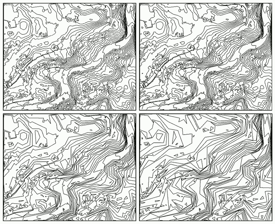
Examples of contours and simplifications are given in Figure 0.6.
Classifying
CGAL provides a package Classification which can be used to segment a point cloud into a user-defined label set. The state-of-the-art classifier currently available in CGAL is the random forest from ETHZ. As it is a supervised classifier, a training set is needed.
The following snippet shows how to use some manually selected training set to train a random forest classifier and compute a classification regularized by a graph cut algorithm:
Point_set::Property_map<int> training_map;
bool training_found;
std::tie (training_map, training_found) = points.property_map<int>("training");
if (training_found)
{
std::cerr << "Classifying ground/vegetation/building" << std::endl;
Classification::Label_set labels ({ "ground", "vegetation", "building" });
Classification::Point_set_feature_generator<Kernel, Point_set, Point_set::Point_map>
generator (points, points.point_map(), 5);
#ifdef CGAL_LINKED_WITH_TBB
features.begin_parallel_additions();
generator.generate_point_based_features (features);
features.end_parallel_additions();
#else
generator.generate_point_based_features (features);
#endif
Classification::ETHZ::Random_forest_classifier classifier (labels, features);
classifier.train (points.range(training_map));
Point_set::Property_map<int> label_map = points.add_property_map<int>("labels").first;
Classification::classify_with_graphcut<Concurrency_tag>
(points, points.point_map(), labels, classifier,
generator.neighborhood().k_neighbor_query(12),
0.5f,
12,
label_map);
std::cerr << "Mean IoU on training data = "
<< Classification::Evaluation(labels,
points.range(training_map),
points.range(label_map)).mean_intersection_over_union() << std::endl;
std::ofstream classified_ofile ("classified.ply");
classified_ofile << points;
classified_ofile.close();
}
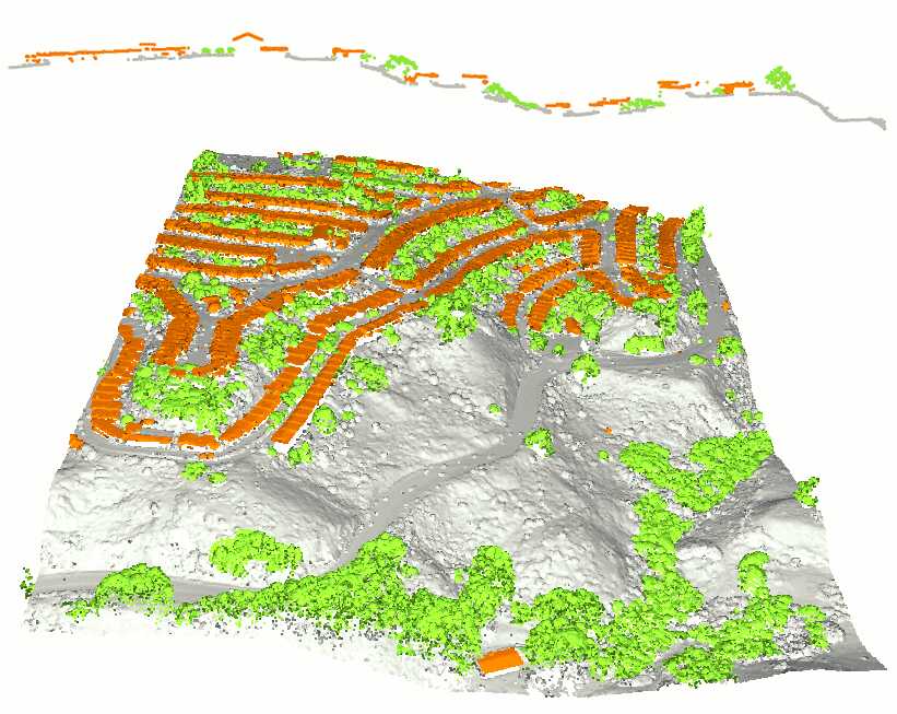
An example of training set and resulting classification is given in Figure 0.7.
Full Code Example
All the code snippets used in this tutorial can be assembled to create a full GIS pipeline (provided the correct includes are used). We give a full code example which achieves all the steps described in this tutorial.
#include <CGAL/Exact_predicates_inexact_constructions_kernel.h>
#include <CGAL/Projection_traits_xy_3.h>
#include <CGAL/Delaunay_triangulation_2.h>
#include <CGAL/Triangulation_vertex_base_with_info_2.h>
#include <CGAL/Triangulation_face_base_with_info_2.h>
#include <CGAL/boost/graph/graph_traits_Delaunay_triangulation_2.h>
#include <CGAL/boost/graph/copy_face_graph.h>
#include <CGAL/Point_set_3.h>
#include <CGAL/Point_set_3/IO.h>
#include <CGAL/compute_average_spacing.h>
#include <CGAL/Surface_mesh.h>
#include <CGAL/Polygon_mesh_processing/locate.h>
#include <CGAL/Polygon_mesh_processing/triangulate_hole.h>
#include <CGAL/Polygon_mesh_processing/border.h>
#include <CGAL/Polygon_mesh_processing/remesh.h>
#include <boost/graph/adjacency_list.hpp>
#include <CGAL/boost/graph/split_graph_into_polylines.h>
#include <CGAL/IO/WKT.h>
#include <CGAL/Constrained_Delaunay_triangulation_2.h>
#include <CGAL/Constrained_triangulation_plus_2.h>
#include <CGAL/Polyline_simplification_2/simplify.h>
#include <CGAL/Polyline_simplification_2/Squared_distance_cost.h>
#include <CGAL/Classification.h>
#include <CGAL/Random.h>
#include <fstream>
#include <queue>
#include "include/Color_ramp.h"
#ifdef CGAL_LINKED_WITH_TBB
#else
#endif
bool face_has_isovalue (TIN::Face_handle fh, double isovalue)
{
bool above = false, below = false;
for (int i = 0; i < 3; ++ i)
{
if (fh->vertex(i)->point().z() > isovalue)
above = true;
if (fh->vertex(i)->point().z() < isovalue)
below = true;
}
return (above && below);
}
Segment_3 isocontour_in_face (TIN::Face_handle fh, double isovalue)
{
Point_3 source;
Point_3 target;
bool source_found = false;
for (int i = 0; i < 3; ++ i)
{
Point_3 p0 = fh->vertex((i+1) % 3)->point();
Point_3 p1 = fh->vertex((i+2) % 3)->point();
if ((p0.z() - isovalue) * (p1.z() - isovalue) > 0)
continue;
double zbottom = p0.z();
double ztop = p1.z();
if (zbottom > ztop)
{
}
double ratio = (isovalue - zbottom) / (ztop - zbottom);
if (source_found)
target = p;
else
{
source = p;
source_found = true;
}
}
return Segment_3 (source, target);
}
template <typename Graph>
class Polylines_visitor
{
private:
std::vector<std::vector<Point_3> >& polylines;
Graph& graph;
public:
Polylines_visitor (Graph& graph, std::vector<std::vector<Point_3> >& polylines)
: polylines (polylines), graph(graph) { }
void start_new_polyline()
{
polylines.push_back (std::vector<Point_3>());
}
void add_node (typename Graph::vertex_descriptor vd)
{
polylines.back().push_back (graph[vd]);
}
void end_polyline()
{
if (polylines.back().size() < 50)
polylines.pop_back();
}
};
using CDT_vertex_base = PS::Vertex_base_2<Projection_traits>;
int main (int argc, char** argv)
{
if (argc != 2)
{
std::cerr << "Usage: " << argv[0] << " points.ply" << std::endl;
std::cerr << "Running with default value " << fname << "\n";
}
std::ifstream ifile (fname, std::ios_base::binary);
ifile >> points;
std::cerr << points.size() << " point(s) read" << std::endl;
TIN dsm (points.points().begin(), points.points().end());
Mesh dsm_mesh;
std::ofstream dsm_ofile ("dsm.ply", std::ios_base::binary);
dsm_ofile.close();
auto idx_to_point_with_info
= [&](const Point_set::Index& idx) -> std::pair<Point_3, Point_set::Index>
{
return std::make_pair (points.point(idx), idx);
};
TIN_with_info tin_with_info
(boost::make_transform_iterator (points.begin(), idx_to_point_with_info),
boost::make_transform_iterator (points.end(), idx_to_point_with_info));
double spacing = CGAL::compute_average_spacing<Concurrency_tag>(points, 6);
spacing *= 2;
auto face_height
= [&](const TIN_with_info::Face_handle fh) -> double
{
double out = 0.;
for (int i = 0; i < 3; ++ i)
out = (
std::max) (out,
CGAL::abs(fh->vertex(i)->point().z() - fh->vertex((i+1)%3)->point().z()));
return out;
};
for (TIN_with_info::Face_handle fh : tin_with_info.all_face_handles())
if (tin_with_info.is_infinite(fh) || face_height(fh) > spacing)
fh->info() = -2;
else
fh->info() = -1;
std::vector<int> component_size;
for (TIN_with_info::Face_handle fh : tin_with_info.finite_face_handles())
{
if (fh->info() != -1)
continue;
std::queue<TIN_with_info::Face_handle> todo;
todo.push(fh);
int size = 0;
while (!todo.empty())
{
TIN_with_info::Face_handle current = todo.front();
todo.pop();
if (current->info() != -1)
continue;
current->info() = int(component_size.size());
++ size;
for (int i = 0; i < 3; ++ i)
todo.push (current->neighbor(i));
}
component_size.push_back (size);
}
std::cerr << component_size.size() << " connected component(s) found" << std::endl;
Mesh tin_colored_mesh;
Mesh::Property_map<Mesh::Face_index, CGAL::IO::Color>
color_map = tin_colored_mesh.add_property_map<Mesh::Face_index,
CGAL::IO::Color>(
"f:color").first;
CGAL::parameters::face_to_face_output_iterator
(boost::make_function_output_iterator
([&](const std::pair<TIN_with_info::Face_handle, Mesh::Face_index>& ff)
{
if (ff.first->info() < 0)
else
{
r.get_int(64, 192),
r.get_int(64, 192));
}
})));
std::ofstream tin_colored_ofile ("colored_tin.ply", std::ios_base::binary);
tin_colored_ofile.close();
int min_size = int(points.size() / 2);
std::vector<TIN_with_info::Vertex_handle> to_remove;
for (TIN_with_info::Vertex_handle vh : tin_with_info.finite_vertex_handles())
{
TIN_with_info::Face_circulator circ = tin_with_info.incident_faces (vh),
start = circ;
bool keep = false;
do
{
if (circ->info() >= 0 && component_size[std::size_t(circ->info())] > min_size)
{
keep = true;
break;
}
}
while (++ circ != start);
if (!keep)
to_remove.push_back (vh);
}
std::cerr << to_remove.size() << " vertices(s) will be removed after filtering" << std::endl;
for (TIN_with_info::Vertex_handle vh : to_remove)
tin_with_info.remove (vh);
Mesh dtm_mesh;
std::vector<Mesh::Face_index> face_selection;
Mesh::Property_map<Mesh::Face_index, bool> face_selection_map
= dtm_mesh.add_property_map<Mesh::Face_index, bool>("is_selected", false).first;
CGAL::parameters::face_to_face_output_iterator
(boost::make_function_output_iterator
([&](const std::pair<TIN_with_info::Face_handle, Mesh::Face_index>& ff)
{
double longest_edge = 0.;
bool border = false;
for (int i = 0; i < 3; ++ i)
{
(ff.first->vertex((i+1)%3)->point(),
ff.first->vertex((i+2)%3)->point()));
TIN_with_info::Face_circulator circ
= tin_with_info.incident_faces (ff.first->vertex(i)),
start = circ;
do
{
if (tin_with_info.is_infinite (circ))
{
border = true;
break;
}
}
while (++ circ != start);
if (border)
break;
}
if (!border && longest_edge > limit)
{
face_selection_map[ff.second] = true;
face_selection.push_back (ff.second);
}
})));
std::ofstream dtm_ofile ("dtm.ply", std::ios_base::binary);
dtm_ofile.close();
std::cerr << face_selection.size() << " face(s) are selected for removal" << std::endl;
face_selection.clear();
for (Mesh::Face_index fi : faces(dtm_mesh))
if (face_selection_map[fi])
face_selection.push_back(fi);
std::cerr << face_selection.size() << " face(s) are selected for removal after expansion" << std::endl;
for (Mesh::Face_index fi : face_selection)
dtm_mesh.collect_garbage();
if (!dtm_mesh.is_valid())
std::cerr << "Invalid mesh!" << std::endl;
std::ofstream dtm_holes_ofile ("dtm_with_holes.ply", std::ios_base::binary);
dtm_holes_ofile.close();
std::vector<Mesh::Halfedge_index> holes;
std::cerr << holes.size() << " hole(s) identified" << std::endl;
double max_size = 0.;
Mesh::Halfedge_index outer_hull;
for (Mesh::Halfedge_index hi : holes)
{
{
const Point_3& p = dtm_mesh.point(target(haf, dtm_mesh));
hole_bbox += p.bbox();
}
Point_2(hole_bbox.
xmax(), hole_bbox.
ymax()));
if (size > max_size)
{
max_size = size;
outer_hull = hi;
}
}
for (Mesh::Halfedge_index hi : holes)
if (hi != outer_hull)
std::ofstream dtm_filled_ofile ("dtm_filled.ply", std::ios_base::binary);
dtm_filled_ofile.close();
std::ofstream dtm_remeshed_ofile ("dtm_remeshed.ply", std::ios_base::binary);
dtm_remeshed_ofile.close();
TIN dtm_clean (dtm_mesh.points().begin(), dtm_mesh.points().end());
CGAL::Bbox_3 bbox = CGAL::bbox_3 (points.points().begin(), points.points().end());
std::size_t width = 1920;
std::size_t height = std::size_t((bbox.ymax() - bbox.ymin()) * 1920 / (bbox.xmax() - bbox.xmin()));
std::cerr << "Rastering with resolution " << width << "x" << height << std::endl;
std::ofstream raster_ofile ("raster.ppm", std::ios_base::binary);
raster_ofile << "P6" << std::endl
<< width << " " << height << std::endl
<< 255 << std::endl;
Color_ramp color_ramp;
TIN::Face_handle location;
for (std::size_t y = 0; y < height; ++ y)
for (std::size_t x = 0; x < width; ++ x)
{
Point_3 query (bbox.xmin() + x * (bbox.xmax() - bbox.xmin()) / double(width),
bbox.ymin() + (height-y) * (bbox.ymax() - bbox.ymin()) / double(height),
0);
location = dtm_clean.locate (query, location);
std::array<unsigned char, 3> colors { 0, 0, 0 };
if (!dtm_clean.is_infinite(location))
{
std::array<double, 3> barycentric_coordinates
(Point_2 (location->vertex(0)->point().x(), location->vertex(0)->point().y()),
Point_2 (location->vertex(1)->point().x(), location->vertex(1)->point().y()),
Point_2 (location->vertex(2)->point().x(), location->vertex(2)->point().y()),
Point_2 (query.x(), query.y()),
Kernel());
double height_at_query
= (barycentric_coordinates[0] * location->vertex(0)->point().z()
+ barycentric_coordinates[1] * location->vertex(1)->point().z()
+ barycentric_coordinates[2] * location->vertex(2)->point().z());
double height_ratio = (height_at_query - bbox.zmin()) / (bbox.zmax() - bbox.zmin());
colors = color_ramp.get(height_ratio);
}
raster_ofile.write (reinterpret_cast<char*>(&colors), 3);
}
raster_ofile.close();
double gaussian_variance = 4 * spacing * spacing;
for (TIN::Vertex_handle vh : dtm_clean.finite_vertex_handles())
{
double z = vh->point().z();
double total_weight = 1;
TIN::Vertex_circulator circ = dtm_clean.incident_vertices (vh),
start = circ;
do
{
if (!dtm_clean.is_infinite(circ))
{
double weight = std::exp(- sq_dist / gaussian_variance);
z += weight * circ->point().z();
total_weight += weight;
}
}
while (++ circ != start);
z /= total_weight;
vh->point() = Point_3 (vh->point().x(), vh->point().y(), z);
}
std::array<double, 50> isovalues;
for (std::size_t i = 0; i < isovalues.size(); ++ i)
isovalues[i] = bbox.zmin() + ((i+1) * (bbox.zmax() - bbox.zmin()) / (isovalues.size() - 2));
using Segment_graph = boost::adjacency_list<boost::listS, boost::vecS, boost::undirectedS, Point_3>;
Segment_graph graph;
using Map_p2v = std::map<Point_3, Segment_graph::vertex_descriptor>;
Map_p2v map_p2v;
for (TIN::Face_handle vh : dtm_clean.finite_face_handles())
for (double iv : isovalues)
if (face_has_isovalue (vh, iv))
{
Segment_3 segment = isocontour_in_face (vh, iv);
for (const Point_3& p : { segment.source(), segment.target() })
{
Map_p2v::iterator iter;
bool inserted;
std::tie (iter, inserted) = map_p2v.insert (std::make_pair (p, Segment_graph::vertex_descriptor()));
if (inserted)
{
iter->second = boost::add_vertex (graph);
graph[iter->second] = p;
}
}
boost::add_edge (map_p2v[segment.source()], map_p2v[segment.target()], graph);
}
std::vector<std::vector<Point_3> > polylines;
Polylines_visitor<Segment_graph> visitor (graph, polylines);
std::cerr << polylines.size() << " polylines computed, with "
<< map_p2v.size() << " vertices in total" << std::endl;
std::ofstream contour_ofile ("contour.wkt");
contour_ofile.precision(18);
contour_ofile.close();
CTP ctp;
for (const std::vector<Point_3>& poly : polylines)
ctp.insert_constraint (poly.begin(), poly.end());
PS::simplify (ctp, PS::Squared_distance_cost(), PS::Stop_above_cost_threshold (16 * spacing * spacing));
polylines.clear();
for (CTP::Constraint_id cid : ctp.constraints())
{
polylines.push_back (std::vector<Point_3>());
polylines.back().reserve (ctp.vertices_in_constraint (cid).size());
for (CTP::Vertex_handle vh : ctp.vertices_in_constraint(cid))
polylines.back().push_back (vh->point());
}
std::size_t nb_vertices
= std::accumulate (polylines.begin(), polylines.end(), std::size_t(0),
[](std::size_t size, const std::vector<Point_3>& poly) -> std::size_t
{ return size + poly.size(); });
std::cerr << nb_vertices
<< " vertices remaining after simplification ("
<< 100. * (nb_vertices / double(map_p2v.size())) << "%)" << std::endl;
std::ofstream simplified_ofile ("simplified.wkt");
simplified_ofile.precision(18);
simplified_ofile.close();
Point_set::Property_map<int> training_map;
bool training_found;
std::tie (training_map, training_found) = points.property_map<int>("training");
if (training_found)
{
std::cerr << "Classifying ground/vegetation/building" << std::endl;
Classification::Label_set labels ({ "ground", "vegetation", "building" });
Classification::Point_set_feature_generator<Kernel, Point_set, Point_set::Point_map>
generator (points, points.point_map(), 5);
#ifdef CGAL_LINKED_WITH_TBB
features.begin_parallel_additions();
generator.generate_point_based_features (features);
features.end_parallel_additions();
#else
generator.generate_point_based_features (features);
#endif
Classification::ETHZ::Random_forest_classifier classifier (labels, features);
classifier.train (points.range(training_map));
Point_set::Property_map<int> label_map = points.add_property_map<int>("labels").first;
Classification::classify_with_graphcut<Concurrency_tag>
(points, points.point_map(), labels, classifier,
generator.neighborhood().k_neighbor_query(12),
0.5f,
12,
label_map);
std::cerr << "Mean IoU on training data = "
<< Classification::Evaluation(labels,
points.range(training_map),
points.range(label_map)).mean_intersection_over_union() << std::endl;
std::ofstream classified_ofile ("classified.ply");
classified_ofile << points;
classified_ofile.close();
}
return EXIT_SUCCESS;
}
References
This tutorial is based on the following CGAL packages:
The data set used throughout this tutorial comes from the https://www.usgs.gov/ database, licensed under the US Government Public Domain.


 1.8.13