
|
CGAL 6.2 - Polygon Mesh Processing
|
Loading...
Searching...
No Matches
|
CGAL 6.2 - Polygon Mesh Processing
|
This package provides a comprehensive set of methods and classes for polygon mesh processing, ranging from basic operations on mesh elements to advanced geometry processing algorithms. The implementation is primarily based on the algorithms and references presented in Botsch et al.'s book on polygon mesh processing [2].
A polygon mesh is a consistent and orientable surface mesh, that can have one or more boundaries. The faces are simple polygons. The edges are segments. Each edge connects two vertices, and is shared by two faces (including the null face for boundary edges). A polygon mesh can have any number of connected components. In this package, a polygon mesh is considered to have the topology of a 2-manifold. Note that all these requirements are mostly combinatorial, and do not impose any geometric constraints on the shape of the polygons. As such, this definition does not prevent the presence of defects such as self-intersections, degenerate faces or edges, etc.
This package follows the BGL API described in CGAL and the Boost Graph Library. It can thus be used either with CGAL::Surface_mesh, CGAL::Polyhedron_3, or any class model of the concept FaceGraph. Each function or class of this package details the requirements on the input polygon mesh.
Named Parameters are used to deal with optional parameters. The page Named Parameters describes their usage.
The algorithms described in this manual are organized in sections:
In all functions of this package, the polygon meshes are required to be models of the graph concepts defined in the package CGAL and the Boost Graph Library. Using common graph concepts enables having common input/output functions for all the models of these concepts. The page I/O Functions provides an exhaustive description of the available I/O functions.
In addition, this package offers the function CGAL::Polygon_mesh_processing::IO::read_polygon_mesh(), which can perform some repairing if the input data do not represent a manifold surface.
This package provides several predicates to determine the characteristics of a triangle mesh or a subset of its faces.
Intersection tests between triangle meshes and/or polylines can be performed using the function CGAL::Polygon_mesh_processing::do_intersect() . Additionally, the function CGAL::Polygon_mesh_processing::intersecting_meshes() can be used to collect all pairs of intersecting meshes within a range.
Self-intersections within a triangle mesh can be detected by calling the function CGAL::Polygon_mesh_processing::does_self_intersect(). Additionally, the function CGAL::Polygon_mesh_processing::self_intersections() reports all pairs of intersecting triangles.
The following example demonstrates self-intersection detection in the pig.off mesh. Detected self-intersections are illustrated in Figure 75.2.
Example: Polygon_mesh_processing/self_intersections_example.cpp
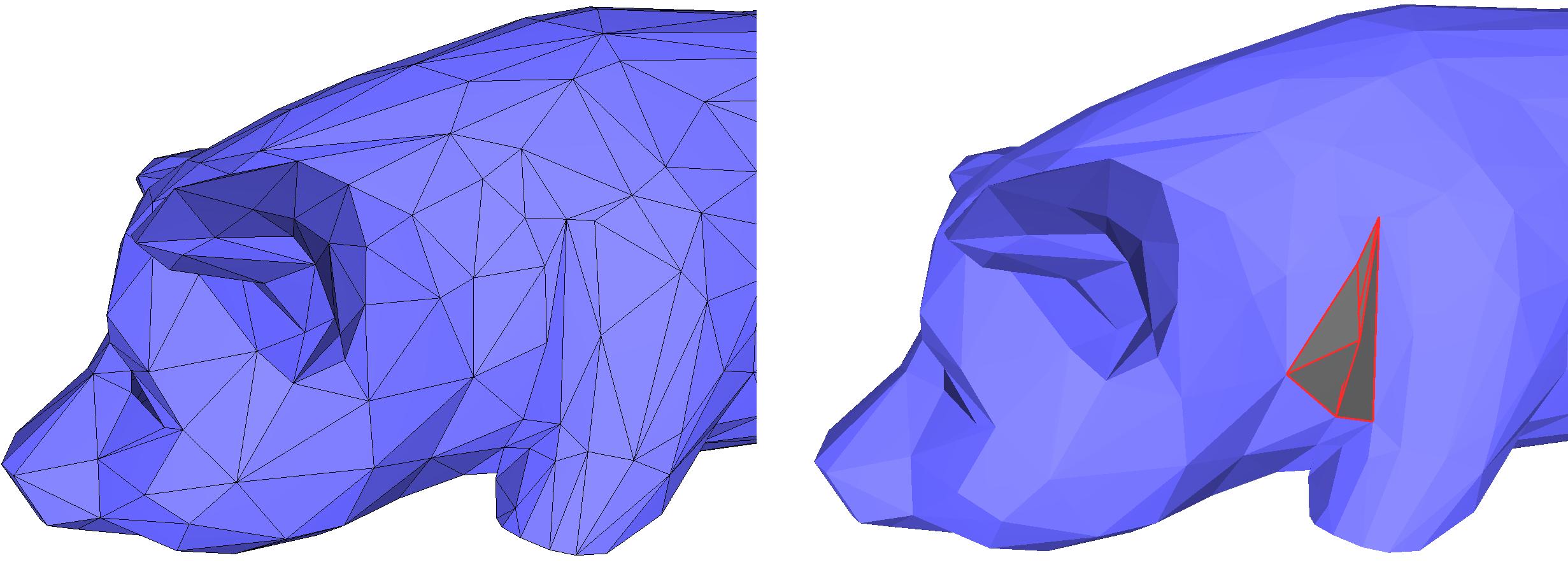
Figure 75.2 Detection of self-intersections in a triangle mesh. Intersecting triangles are displayed in dark grey and red in the right image.
The class CGAL::Side_of_triangle_mesh provides a functor that can answer whether a query point is inside, outside, or on the boundary of the domain bounded by a given closed triangle mesh.
A point is considered to be on the bounded side of the mesh if an odd number of surfaces are crossed when moving from the point to infinity.
The algorithm can handle the case of a triangle mesh with several connected components, but is expected to contain no self-intersections. In case of self-inclusions, the ray intersections parity test is performed, and the execution will not fail. However, users should be aware that the predicate alternately considers sub-volumes to be on the bounded and unbounded sides of the input triangle mesh.
Example: Polygon_mesh_processing/point_inside_example.cpp
The class CGAL::Polyhedral_envelope provides functors to check whether a query point, segment, or triangle is fully contained within a polyhedral envelope of a triangle mesh or triangle soup.
A polyhedral envelope is a conservative approximation of the Minkowski sum envelope of a set of triangles with a sphere of radius \( \epsilon \). The Minkowski sum envelope features cylindrical and spherical patches at convex edges and vertices.
Given a distance \( \delta = \epsilon / \sqrt(3)\), a prism is associated with each triangle by intersecting halfspaces parallel and orthogonal to the triangle and its edges, and additional halfspaces for obtuse angles, with face normals corresponding to angle bisectors. These halfspaces are at distance \( \delta \) and contain the triangle.
The polyhedral envelope of a set of triangles with a tolerance \( \epsilon \) then is the union of the prisms of all faces with \( \delta = \epsilon / \sqrt(3) \).
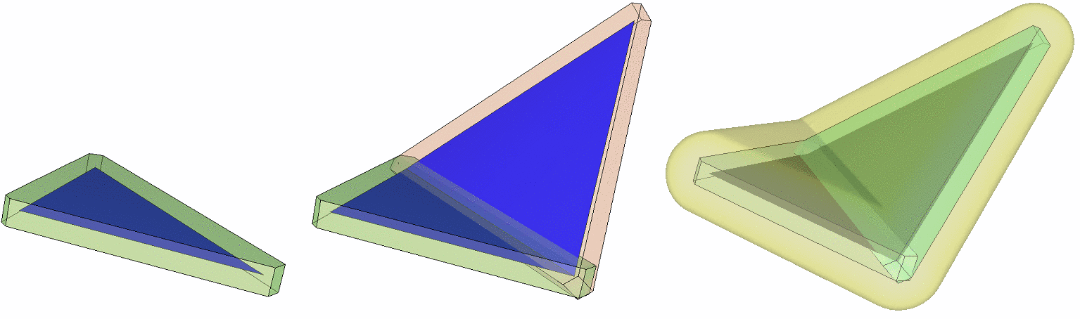
Figure 75.3 The prism for a single triangle (left), the polyhedral envelope (middle), and the Minkowski sum envelope (right) for a triangle mesh.
The polyhedral envelope is guaranteed to be contained within the Minkowski sum envelope. The containment test is exact for the polyhedral envelope and conservative for the Minkowski sum envelope: if a query is inside the polyhedral envelope, it is also inside the Minkowski sum envelope; if outside, its relation to the Minkowski sum envelope is undetermined.
The algorithm of Wang et al. [8] for polyhedral envelope containment proceeds as follows:
The prisms of the faces of the input triangles are stored in an AABB tree, which is used to quickly identify the prisms whose bounding box overlaps with the query.
For a query point, the algorithm checks if it is inside one of these prisms. For a query segment or triangle, the algorithm checks if the query is completely covered. The details of how to check this covering can be found in the paper.
Polyhedral envelope containment is used by Surface_mesh_simplification::Polyhedral_envelope_filter in the Triangulated Surface Mesh Simplification package to simplify triangle meshes within a given tolerance.
The following example demonstrates construction of a polyhedral envelope for a CGAL::Surface_mesh and performing queries.
Example: Polygon_mesh_processing/polyhedral_envelope.cpp
As connectivity information is not required, the same check can be performed on a triangle soup.
Example: Polygon_mesh_processing/polyhedral_envelope_of_triangle_soup.cpp
A triangle mesh can also be used as a query to verify if a remeshed version is contained within the polyhedral envelope of an input mesh.
Example: Polygon_mesh_processing/polyhedral_envelope_mesh_containment.cpp
Badly shaped or, even worse, completely degenerate elements of a polygon mesh are problematic in many algorithms which one might want to use on the mesh. This package offers a toolkit of functions to detect such undesirable elements.
CGAL::Polygon_mesh_processing::is_degenerate_edge(), to detect if an edge is degenerate (that is, if its two vertices share the same geometric location).CGAL::Polygon_mesh_processing::is_degenerate_triangle_face(), to detect if a face is degenerate (that is, if its three vertices are collinear).CGAL::Polygon_mesh_processing::degenerate_edges(), to collect degenerate edges within a range of edges.CGAL::Polygon_mesh_processing::degenerate_faces(), to collect degenerate faces within a range of faces.CGAL::Polygon_mesh_processing::is_cap_triangle_face(), to detect if a face has one very large angle.CGAL::Polygon_mesh_processing::is_needle_triangle_face(), to detect if a face has a very short edge.Functions are provided to enumerate and store the connected components of a polygon mesh. Connected components may be closed and geometrically separated, or separated by border or user-specified constraint edges.
The main entry point is the function CGAL::Polygon_mesh_processing::connected_components(), which collects all the connected components and fills a property map with the indices of the different connected components.
If a single connected component is to be extracted, the function CGAL::Polygon_mesh_processing::connected_component() collects all the faces that belong to the same connected component as the face that is provided as a parameter.
When a mesh has no boundary, it partitions the 3D space in different volumes. The function CGAL::Polygon_mesh_processing::volume_connected_components() can be used to assign to each face an id per volume defined by the surface connected components.
It is often useful to retain or remove specific connected components, for example, to discard small noisy components in favor of larger ones.
The functions CGAL::Polygon_mesh_processing::keep_connected_components() and CGAL::Polygon_mesh_processing::remove_connected_components() enable the user to keep or remove only a selection of connected components, provided either as a range of faces that belong to the desired connected components or as a range of connected component ids (one or more per connected component).
Finally, it can be useful to quickly remove some connected components based on characteristics of the surface mesh. The function CGAL::Polygon_mesh_processing::keep_largest_connected_components() enables the user to keep only a given number from the largest connected components. The size of a connected component is given by the sum of the sizes of the faces it contains; by default, the size of a face is 1, and thus the size of a connected component is equal to the number of faces it contains. However, it is also possible to pass a face size map, such that the size of the face is its area, for example. Similarly to the previous function, the function CGAL::Polygon_mesh_processing::keep_large_connected_components() can be used to discard all connected components whose size is below a user-defined threshold.
Finally, CGAL::Polygon_mesh_processing::split_connected_components() splits the mesh into separate meshes for each connected component.
The first example shows how to record the connected components of a polygon mesh. In particular, we provide an example for the optional parameter EdgeConstraintMap, a property map that returns information about an edge being a constraint or not. A constraint provides a means to demarcate the border of a connected component, and prevents the propagation of a connected component index to cross it.
Example: Polygon_mesh_processing/connected_components_example.cpp
The second example shows how to use the class template Face_filtered_graph, which enables treating one or several connected components as a separate face graph.
Example: Polygon_mesh_processing/face_filtered_graph_example.cpp
To ease the manipulation of points on a surface, CGAL offers a multitude of functions based upon a different representation of a point on a polygon mesh: the point is represented as a pair of a face of the polygon mesh and a triplet of barycentric coordinates. This definition enables a robust handling of polylines between points living in the same face: for example, two 3D segments created by four points within the same face that should intersect might not actually intersect due to inexact computations. However, manipulating these same points through their barycentric coordinates can instead be done, and intersections computed in the barycentric space will not suffer from the same issues. Furthermore, this definition is only dependent on the intrinsic dimension of the surface (i.e. 2) and not on the ambient dimension within which the surface is embedded.
The functions of the group Location Functions offer the following functionalities:
CGAL::Polygon_mesh_processing::locate() and similar,CGAL::Polygon_mesh_processing::locate_with_AABB_tree() and similar,CGAL::Polygon_mesh_processing::is_on_face_border() and similar.The following example demonstrates usage of these functions.
Example: Polygon_mesh_processing/locate_example.cpp
Methods are provided to compute normals on polygon meshes, either per face or per vertex:
CGAL::Polygon_mesh_processing::compute_face_normal()CGAL::Polygon_mesh_processing::compute_vertex_normal()When computing all the normals of faces and vertices, the following functions should be preferred as they factorize some computations:
CGAL::Polygon_mesh_processing::compute_face_normals()CGAL::Polygon_mesh_processing::compute_vertex_normals()CGAL::Polygon_mesh_processing::compute_normals()In the following examples we associate a normal vector to each vertex and to each face of a mesh of type CGAL::Surface_mesh.
Example: Polygon_mesh_processing/compute_normals_example.cpp
This package provides methods to compute curvatures on polygon meshes based on "Interpolated Corrected Curvatures on Polyhedral Surfaces" [4]. This includes mean curvature, Gaussian curvature, principal curvatures and directions. These can be computed on triangle meshes, quad meshes, and meshes with n-gon faces (for n-gons, the centroid must be inside the n-gon face). The algorithms used prove to work well in general. Furthermore, they give accurate results on meshes with noise on vertex positions, under the condition that the correct vertex normals are provided.
It is worth noting that the Principal Curvatures and Directions can also be estimated using the Estimation of Local Differential Properties of Point-Sampled Surfaces package, which estimates the local differential quantities of a surface at a point using a local polynomial fitting (fitting a d-jet). Unlike the Interpolated Corrected Curvatures, the Jet Fitting method discards topological information, and thus can be used on point clouds as well.
Surface curvatures are quantities that describe the local geometry of a surface. They are important in many geometry processing applications. As surfaces are 2-dimensional objects (embedded in 3D), they can bend in 2 independent directions. These directions are called principal directions, and the amount of bending in each direction is called the principal curvature: \( k_1 \) and \( k_2 \) (denoting max and min curvatures). Curvature is usually expressed as scalar quantities like the mean curvature \( H \) and the Gaussian curvature \( K \) which are defined in terms of the principal curvatures.
The algorithms are based on the two papers [5] and [4]. They introduce a new way to compute curvatures on polygon meshes. The main idea in [5] is based on decoupling the normal information from the position information, which is useful for dealing with digital surfaces, or meshes with noise on vertex positions. [4] introduces some extensions to this framework, as it uses linear interpolation on the corrected normal vector field to derive new closed-form equations for the corrected curvature measures. These interpolated curvature measures are the first step for computing the curvatures. For a triangle \( \tau_{ijk} \), with vertices i, j, k:
\begin{align*} \mu^{(0)}(\tau_{ijk}) = &\frac{1}{2} \langle \bar{\mathbf{u}} \mid (\mathbf{x}_j - \mathbf{x}_i) \times (\mathbf{x}_k - \mathbf{x}_i) \rangle, \\ \mu^{(1)}(\tau_{ijk}) = &\frac{1}{2} \langle \bar{\mathbf{u}} \mid (\mathbf{u}_k - \mathbf{u}_j) \times \mathbf{x}_i + (\mathbf{u}_i - \mathbf{u}_k) \times \mathbf{x}_j + (\mathbf{u}_j - \mathbf{u}_i) \times \mathbf{x}_k \rangle, \\ \mu^{(2)}(\tau_{ijk}) = &\frac{1}{2} \langle \mathbf{u}_i \mid \mathbf{u}_j \times \mathbf{u}_k \rangle, \\ \mu^{\mathbf{X},\mathbf{Y}}(\tau_{ijk}) = & \frac{1}{2} \big\langle \bar{\mathbf{u}} \big| \langle \mathbf{Y} | \mathbf{u}_k -\mathbf{u}_i \rangle \mathbf{X} \times (\mathbf{x}_j - \mathbf{x}_i) \big\rangle -\frac{1}{2} \big\langle \bar{\mathbf{u}} \big| \langle \mathbf{Y} | \mathbf{u}_j -\mathbf{u}_i \rangle \mathbf{X} \times (\mathbf{x}_k - \mathbf{x}_i) \big\rangle, \end{align*}
where \( \langle \cdot \mid \cdot \rangle \) denotes the scalar product, and \( \bar{\mathbf{u}}=\frac{1}{3}( \mathbf{u}_i + \mathbf{u}_j + \mathbf{u}_k )\).
The first measure \( \mu^{(0)} \) is the area measure of the triangle, and the measures \( \mu^{(1)} \) and \( \mu^{(2)} \) are the mean and Gaussian corrected curvature measures of the triangle. The last measure \( \mu^{\mathbf{X},\mathbf{Y}} \) is the anisotropic corrected curvature measure of the triangle. The anisotropic measure is later used to compute the principal curvatures and directions through an eigenvalue solver.
The interpolated curvature measures are then computed for each vertex \( v \) as the sum of the curvature measures of the faces in a ball around \( v \) weighted by the inclusion ratio of the triangle in the ball. This ball radius is an optional (named) parameter of the function. There are 3 cases for the ball radius passed value:
average_edge_length * 1e-6) is used (to account for the convergence of curvatures at infinitely small balls).To get the final curvature value for a vertex \( v \), the respective interpolated curvature measure is divided by the interpolated area measure.
\[ \mu^{(k)}( B ) = \sum_{\tau : \text{triangle} } \mu^{(k)}( \tau ) \frac{\mathrm{Area}( \tau \cap B )}{\mathrm{Area}(\tau)}. \]
The implementation is generic with respect to mesh data structure and can be used with CGAL::Surface_mesh, CGAL::Polyhedron_3, or any polygon mesh structure meeting the FaceGraph concept requirements.
Curvatures are computed for all vertices using CGAL::Polygon_mesh_processing::interpolated_corrected_curvatures(), with named parameters to select which curvatures (and directions) to compute. An overload is available for computing curvatures at a single vertex.
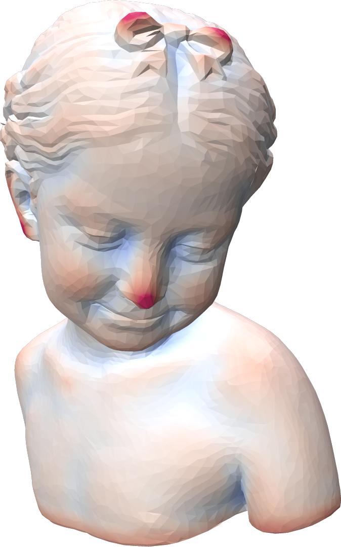
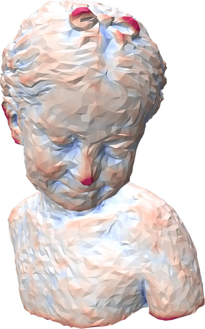
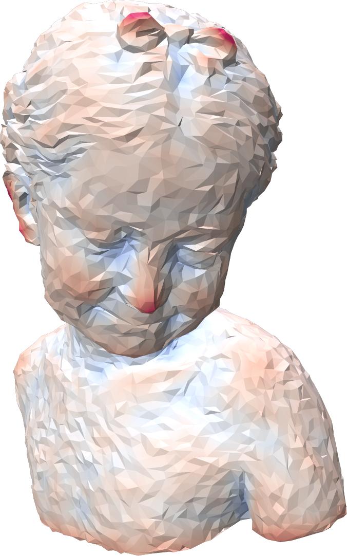
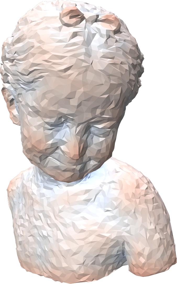
Figure 75.4 illustrates various curvature measures on a triangular mesh.
 | 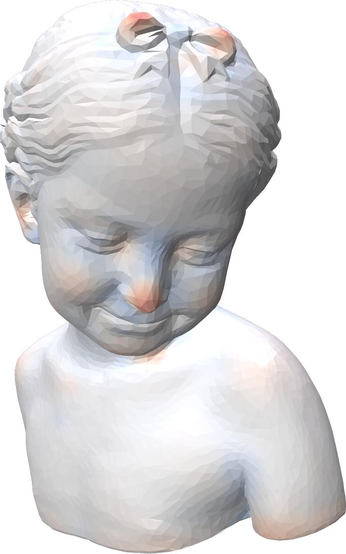 | 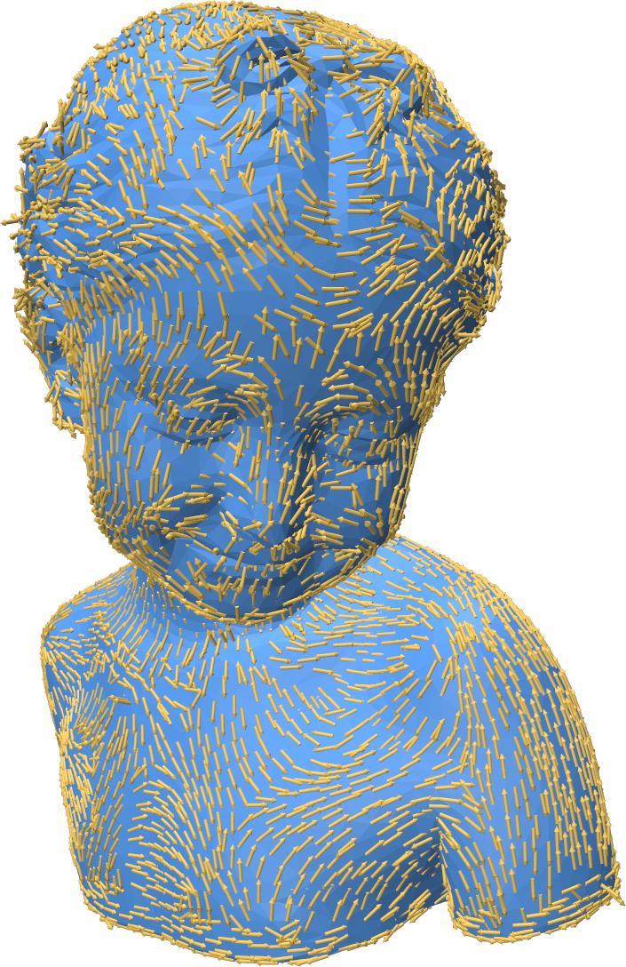 | 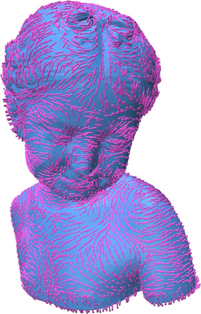 |
| (a) | (b) |
Figure 75.4 Mean curvature, Gaussian curvature, minimal principal curvature direction, and maximal principal curvature direction on a mesh (ball radius set to 0.04).
 |  | |  |
 |  |  |  |
| (a) | (b) |
Figure 75.5 Varying the integration ball radius yields a scale space of curvature measures, useful for handling noise in the input mesh. The second row illustrates mean curvature with fixed colormap ranges and ball radii in {0.02,0.03,0.04,0.05}.
The implemented algorithms exhibit a linear complexity in the number of faces of the mesh. It is worth noting that we pre-computed the vertex normals and passed them as a named parameter to the function to better estimate the performance of the curvature computation. For the data reported in the following table, we used a machine with an Intel Core i7-8750H CPU @ 2.20GHz, 16GB of RAM, on Windows 11, 64 bits and compiled with Visual Studio 2019.
| Ball Radius | Computation | Spot (6k faces) | Bunny (144K faces) | Stanford Dragon (871K faces) | Old Age or Winter (6M faces) |
|---|---|---|---|---|---|
| vertex 1-ring faces (default) | Mean Curvature | < 0.001 s | 0.019 s | 0.11 s | 2.68 s |
| Gaussian Curvature | < 0.001 s | 0.017 s | 0.10 s | 2.77 s | |
| Principal Curvatures & Directions | 0.002 s | 0.044 s | 0.25 s | 3.98 s | |
| All (optimized for shared computations) | 0.003 s | 0.049 s | 0.28 s | 4.52 s | |
| r = 0.1 * avg_edge_length | Mean Curvature | 0.017 s | 0.401 s | 2.66 s | 22.29 s |
| Gaussian Curvature | 0.018 s | 0.406 s | 2.63 s | 21.61 s | |
| Principal Curvatures & Directions | 0.019 s | 0.430 s | 2.85 s | 23.55 s | |
| All (optimized for shared computations) | 0.017 s | 0.428 s | 2.89 s | 24.16 s | |
| r = 0.5 * avg_edge_length | Mean Curvature | 0.024 s | 0.388 s | 3.18 s | 22.79 s |
| Gaussian Curvature | 0.024 s | 0.392 s | 3.21 s | 23.58 s | |
| Principal Curvatures & Directions | 0.027 s | 0.428 s | 3.41 s | 24.44 s | |
| All (optimized for shared computations) | 0.025 s | 0.417 s | 3.44 s | 23.93 s |
Figure 75.6 Performance of the curvature computation on various meshes (in seconds). The first 4 rows show the performance of the default value for the ball radius, which is using the 1-ring of neighboring faces around each vertex, instead of actually approximating the inclusion ratio of the faces in a ball of certain radius. The other rows show a ball radius of 0.1 (and 0.5) scaled by the average edge length of the mesh. It is clear that using the 1-ring of faces is much faster, but it might not be as effective when used on a noisy input mesh.
Property Maps are used to record computed curvatures, as shown in the examples. For each property map, a curvature value is associated with each vertex.
The following example demonstrates computation of curvatures at vertices and storage in property maps provided by CGAL::Surface_mesh.
Example: Polygon_mesh_processing/interpolated_corrected_curvatures_SM.cpp
The following example illustrates how to compute the curvatures on vertices and store them in dynamic property maps as the class CGAL::Polyhedron_3 does not provide storage for the curvatures.
Example: Polygon_mesh_processing/interpolated_corrected_curvatures_PH.cpp
The following example demonstrates computation of curvatures at a specific vertex.
Example: Polygon_mesh_processing/interpolated_corrected_curvatures_vertex.cpp
The package also provides methods to compute the standard, non-interpolated discrete mean and Gaussian curvatures on triangle meshes, based on the work of Meyer et al. [6]. These curvatures are computed at each vertex of the mesh, and are based on the angles of the incident triangles. The functions are:
CGAL::Polygon_mesh_processing::discrete_mean_curvature()CGAL::Polygon_mesh_processing::discrete_mean_curvatures()CGAL::Polygon_mesh_processing::discrete_Gaussian_curvature()CGAL::Polygon_mesh_processing::discrete_Gaussian_curvatures()This package provides methods to detect some features of a polygon mesh.
The function CGAL::Polygon_mesh_processing::sharp_edges_segmentation() detects sharp edges and deduces surface patches and vertex incidences. It is composed of three functions:
CGAL::Polygon_mesh_processing::detect_sharp_edges()CGAL::Polygon_mesh_processing::connected_components()CGAL::Polygon_mesh_processing::detect_vertex_incident_patches()These functions respectively detect sharp edges, compute patch indices, and assign patch indices to each vertex based on incident faces.
The following example counts the number of edges incident to two faces whose normals form an angle less than 90 degrees, and the number of surface patches separated by these edges.
Example: Polygon_mesh_processing/detect_features_example.cpp
This package provides methods to compute (approximate) distances between meshes and point sets.
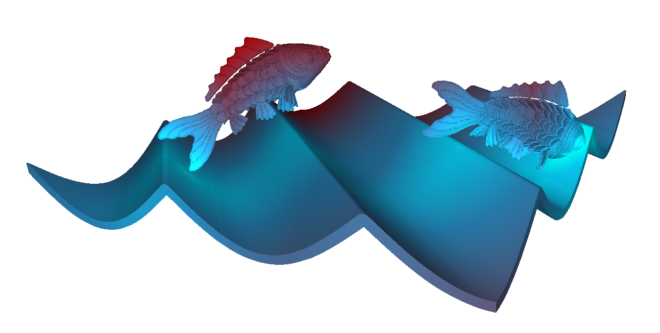
The function approximate_Hausdorff_distance() computes an approximation of the Hausdorff distance from a mesh tm1 to a mesh tm2. Given a a sampling of tm1, it computes the distance to tm2 of the farthest sample point to tm2 [3]. The symmetric version (approximate_symmetric_Hausdorff_distance()) is the maximum of the two non-symmetric distances. Internally, points are sampled using sample_triangle_mesh() and the distance to each sample point is computed using max_distance_to_triangle_mesh(). The quality of the approximation depends on the quality of the sampling and the runtime depends on the number of sample points. Three sampling methods with different parameters are provided (see Figure 75.7).
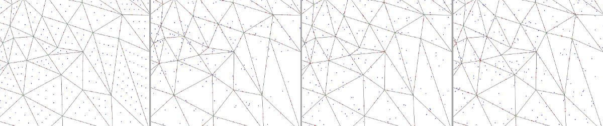
Figure 75.7 Sampling of a triangle mesh using different sampling methods. From left to right: (a) Grid sampling, (b) Monte-Carlo sampling with fixed number of points per face and per edge, (c) Monte-Carlo sampling with a number of points proportional to the area/length, and (d) Uniform random sampling. The four pictures represent the sampling on the same portion of a mesh, parameters were adjusted so that the total number of points sampled in faces (blue points) and on edges (red points) are roughly the same. Note that when using the random uniform sampling some faces/edges may not contain any point, but this method is the only one that allows to exactly match a given number of points.
The function approximate_max_distance_to_point_set() computes an approximation of the Hausdorff distance from a mesh to a point set. For each triangle, lower and upper bounds of the Hausdorff distance to the point set are computed. Triangles are refined until the difference between bounds is below a user-defined precision threshold.
In the following example, a mesh is isotropically remeshed and the approximate distance between the input and the output is computed.
Example: PMP_Remeshing/hausdorff_distance_remeshing_example.cpp
In Poisson_surface_reconstruction_3/poisson_reconstruction_example.cpp, a triangulated surface mesh is constructed from a point set using the Poisson reconstruction algorithm , and the distance between the point set and the reconstructed surface is computed as follows:
The function CGAL::Polygon_mesh_processing::bounded_error_Hausdorff_distance() computes an estimate of the Hausdorff distance of two triangle meshes which is bounded by a user-given error bound. Given two meshes tm1 and tm2, it follows the procedure given by [7]. Namely, a bounded volume hierarchy (BVH) is built on tm1 and tm2 respectively. The BVH on tm1 is used to iterate over all triangles in tm1. Throughout the traversal, the procedure keeps track of a global lower and upper bound on the Hausdorff distance respectively. For each triangle t in tm1, by traversing the BVH on tm2, it is estimated via the global bounds whether t can still contribute to the actual Hausdorff distance. From this process, a set of candidate triangles is selected.
The candidate triangles are subsequently subdivided and for each smaller triangle, the BVH on tm2 is traversed again. This is repeated until the triangle is smaller than the user-given error bound, all vertices of the triangle are projected onto the same triangle in tm2, or the triangle's upper bound is lower than the global lower bound. After creation, the subdivided triangles are added to the list of candidate triangles. Thereby, all candidate triangles are processed until a triangle is found in which the Hausdorff distance is realized or in which it is guaranteed to be realized within the user-given error bound.
In the current implementation, the BVH used is an AABB-tree and not the swept sphere volumes as used in the original implementation. This should explain the runtime difference observed with the original implementation.
The function CGAL::Polygon_mesh_processing::bounded_error_Hausdorff_distance() computes the one-sided Hausdorff distance from tm1 to tm2. This component also provides the symmetric distance CGAL::Polygon_mesh_processing::bounded_error_symmetric_Hausdorff_distance() and a utility function called CGAL::Polygon_mesh_processing::is_Hausdorff_distance_larger() that returns true if the Hausdorff distance between two meshes is larger than the user-defined max distance.
In the following examples: (a) the distance of a tetrahedron to a remeshed version of itself is computed, (b) the distance of two geometries is computed which is realized strictly in the interior of a triangle of the first geometry, (c) a perturbation of a user-given mesh is compared to the original user-given mesh, (d) two user-given meshes are compared, where the second mesh is gradually moved away from the first one.
Example: Polygon_mesh_processing/hausdorff_bounded_error_distance_example.cpp
A first version of this package was started by Ilker O. Yaz and Sébastien Loriot. Jane Tournois worked on the finalization of the API, code, and documentation.
The polyhedral envelope containment check was integrated in CGAL 5.3. The implementation makes use of the version of https://github.com/wangbolun300/fast-envelope available on 7th of October 2020. It only uses the high level algorithm of checking that a query is covered by a set of prisms, where each prism is an offset for an input triangle. That is, the implementation in CGAL does not use indirect predicates.
Interpolated corrected curvatures were implemented during GSoC 2022 by Hossam Saeed, supervised by David Coeurjolly, Jacques-Olivier Lachaud, and Sébastien Loriot. The implementation is based on [4]. DGtal's implementation was also referenced during development.