
|
CGAL 6.2 - 3D Isosurfacing
|
Loading...
Searching...
No Matches
|
CGAL 6.2 - 3D Isosurfacing
|
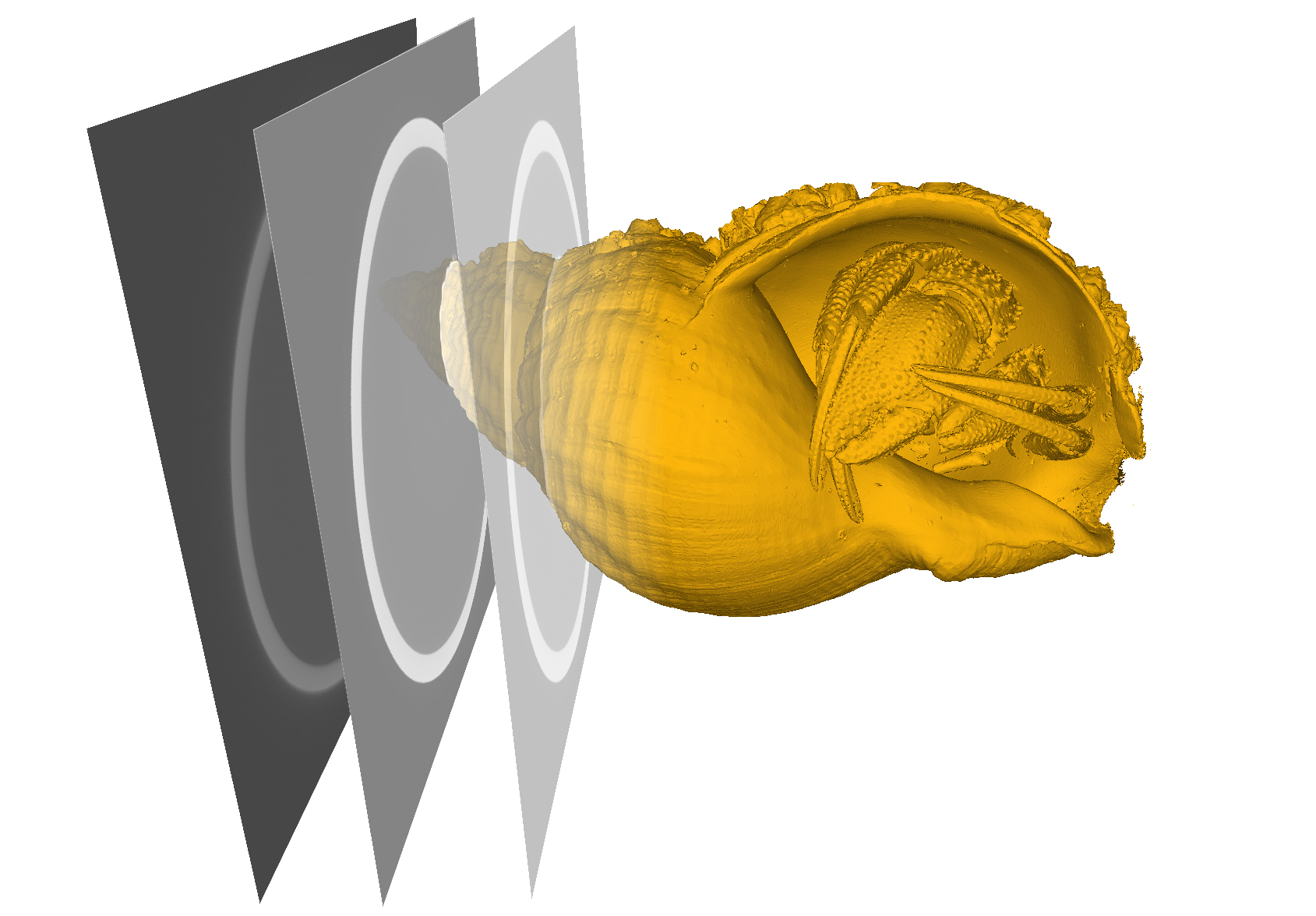
Figure 64.1 Generating a surface from a 3D gray level image using Marching Cubes (3D input image from qim.dk)
Given a field of a scalar values, an isosurface is defined as the locus of points where the field has a given constant value; in other words, it is a level set. This constant value is referred to as the "isovalue", and, for well-behaved fields, the level set forms a surface. In the following, we shall refer to the field of scalar values as the value field. "Isosurfacing", also known as "isosurface extraction" or "contouring", is the process of constructing the isosurface corresponding to a given value field and isovalue. Isosurfacing is often needed for volume visualization and for the simulation of physical phenomena.
This CGAL package provides methods to extract isosurfaces from 3D value fields. These contouring techniques rely on the partition of the 3D space and of the field to construct an approximate representation of the isosurface. The 3D value field can be described through various representations: an implicit function, an interpolated set of discrete sampling values, a 3D image, etc. (see Examples). The isovalue is user-defined. The output is a polygon soup, made either of triangles or quads depending on the method, and may consist of a single connected component, or multiple, disjoint components. Note that due to the inherent approximate nature of these discrete methods that only sample 3D value fields, parts of the "true" isosurface may be missing from the output, and the output may contain artifacts that are not present in the true isosurface.
The scientific literature abounds with algorithms for extracting isosurfaces, each coming with different properties for the output and requirements for the input [2]. This package offers the following methods
Marching Cubes (MC) [6] uses a volumetric grid, i.e., a 3D iso-cuboid partitioned into hexahedral cells. All cells of the grid are processed individually using values of the value field sampled at the grid corners. Each cell corner is assigned a sign (+/-) to indicate whether its value field value is above or below the user-defined isovalue. A vertex is created along each grid edge where a sign change occurs, i.e., where the edge intersects the isosurface. More specifically, the vertex location is computed using linear interpolation of the value field values evaluated at the cell corners forming the edge. These vertices are connected to form triangles within the cell, depending on the configuration of signs at the cell corners. Figure 64.2 illustrates the configurations in 2D. In 3D, there are no less than 33 configurations (not shown) [1].
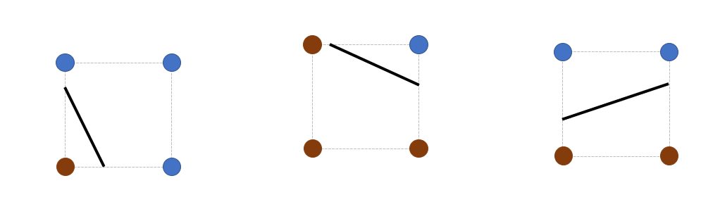
Figure 64.2 Examples of some configurations for 2D Marching Cubes.
The implementation within CGAL is generic in the sense that it can process any grid-like data structure that consists of hexahedral cells. When the hexahedral grid is a conforming grid (meaning that the intersection of two hexahedral cells is a face, an edge, or a vertex), the Marching Cubes algorithm generates as output a surface triangle mesh that is almost always combinatorially 2-manifold, yet can still exhibit topological issues such as holes or non-conforming edges.
If the mesh is 2-manifold and the isosurface does not intersect the domain boundary, then the output mesh is watertight. As the Marching Cubes algorithm uses linear interpolation of the sampled value field along the grid edges, it can miss details or components that are not captured by the sampling of the value field.
Compared to other meshing approaches such as Delaunay refinement, Marching Cubes is substantially faster, but often tends to generate more triangle facets for an equivalent desired sizing field. In addition, the quality of the triangle facets is in general poor, with many needle or cap-shaped triangles.
Furthermore, Marching Cubes does not preserve the sharp features present in the isovalue of the input value field (see Figure 64.4).
Topologically Correct Marching Cubes is an extension to the Marching Cubes algorithm which provides additional guarantees for the output [4]. More specifically, it generates as output a mesh that is homeomorphic to the trilinear interpolant of the input value field inside each cube. This means that the output mesh can accurately represent small complex features. For example, a tunnel of the isosurface within a single cell is topologically resolved. To achieve this, the algorithm can insert additional vertices within cells. Furthermore, the mesh is guaranteed to be 2-manifold and watertight, as long as the isosurface does not intersect the domain boundaries.
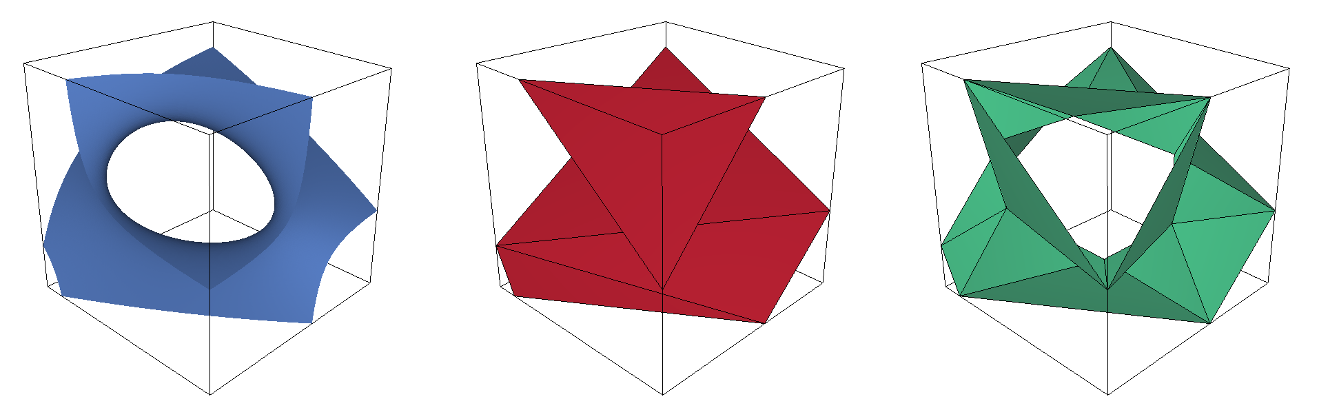
Figure 64.3 Marching Cubes vs Topologically Correct Marching Cubes. Some vertex values can represent complex surfaces within a single cell: on the left, the values at the vertices of the cell have been interpolated within the cell and correspond to a tunnel-like surface. This surface is not correctly recovered when applying the cases of the Marching Cubes algorithm to the cell: 2 independent disk-like sheets are created (middle). However, by inserting new vertices, TMC correctly captures the topology within a single cell (right).
Dual Contouring (DC) [5] is a method that does not generate vertices on the grid edges, but within cells instead. A facet is created for each edge that intersects the isosurface by connecting the vertices of the incident cells. For a uniform hexahedral grid, this results in a quadrilateral surface mesh. Dual Contouring can deal with any domain but guarantees neither a 2-manifold nor a watertight mesh. On the other hand, it generates fewer faces and higher quality faces than Marching Cubes, in general. Finally, its main advantage over Marching Cubes is its ability to recover sharp creases and corners.
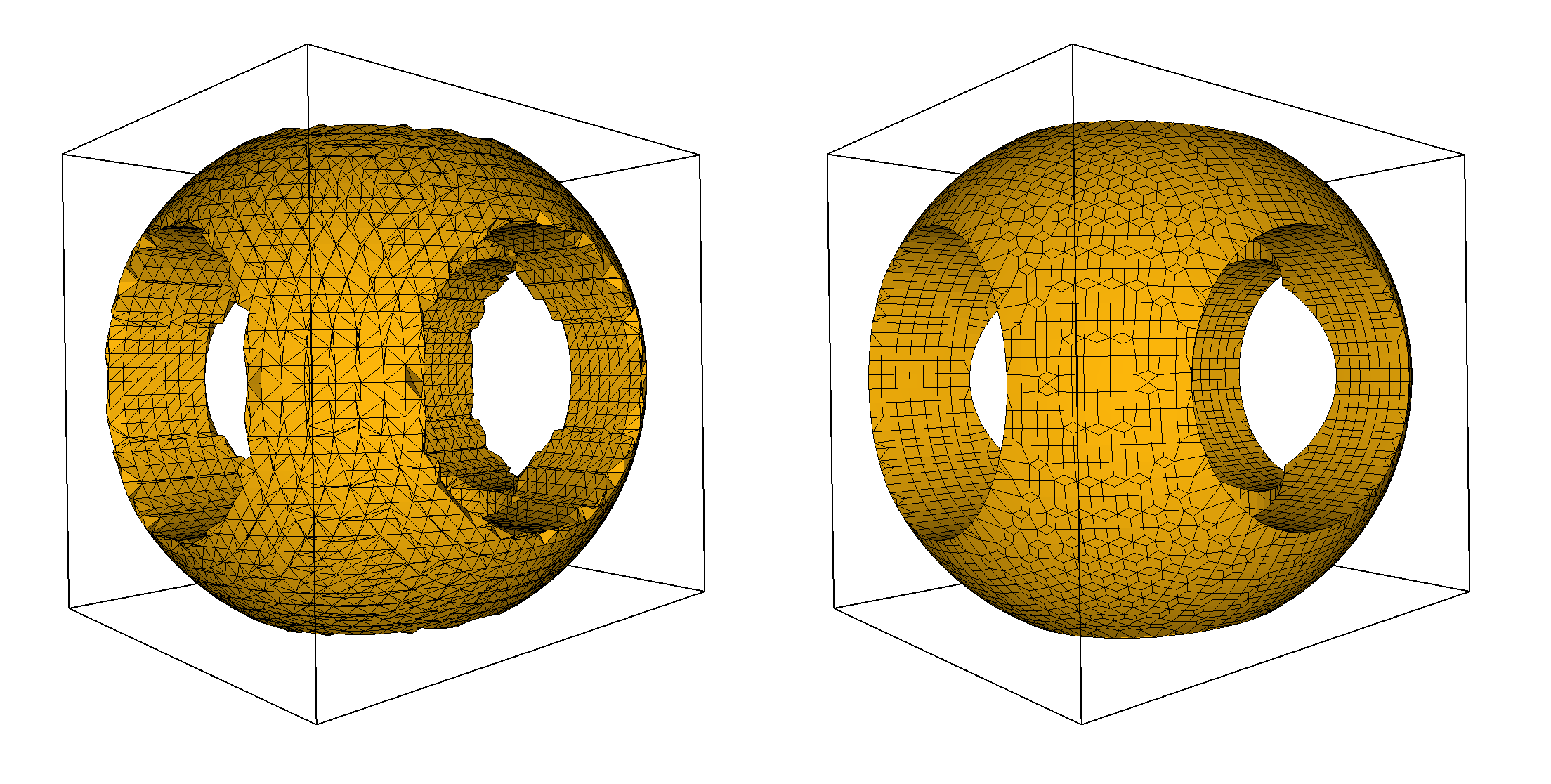
Figure 64.4 Comparison between a mesh of a CSG shape generated by Marching Cubes (left) and Dual Contouring (right).
In addition to the 3D value field, Dual Contouring requires knowledge about the gradient of the value field.
The CGAL implementation uses a vertex positioning strategy based on Quadric Error Metrics [3] : for a cell, the vertex location is computed by minimizing the error to the sum of the quadrics defined at each edge-isosurface intersection. Using this approach, the vertex may be located outside the cell, which is a desirable property to improve the odds of recovering sharp features, but it might also create self-intersections. Users can choose to constrain the vertex location inside the cell.
By default, Dual Contouring generates quads, but using edge-isosurface intersections, one can "star" these quads to generate four triangles. Triangulating the quads is the default behavior in CGAL, but this can be changed using a named parameter.
The following table summarizes the differences between the algorithms in terms of constraints over the input 3D domain, the facets of the output surface mesh, and the properties of the output surface mesh.
| Algorithm | Facets | 2-Manifold | Watertight* | Topologically Correct | Recovery of Sharp Features |
|---|---|---|---|---|---|
| MC | Triangles | no | no | no | no |
| TMC | Triangles | yes | yes | yes | no |
| DC | Quads** | no | no | no | yes (not guaranteed) |
Note that the output mesh has boundaries when the isosurface intersects the domain boundaries, regardless of the method (see Figure 64.5).
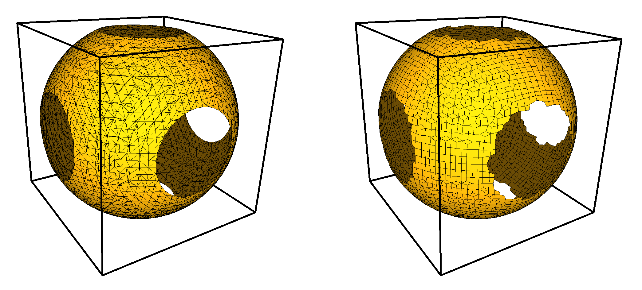
Figure 64.5 Outputs of Marching Cubes (left) and Dual Contouring (right) for an implicit sphere of radius 1.1 and a domain of size 2x2x2, both centered at the origin. Output meshes can have boundaries when the isosurface intersects the domain boundary.
The following functions are the main entry points to the isosurfacing algorithms of this package:
CGAL::Isosurfacing::marching_cubes(), using the named parameter: use_topologically_correct_marching_cubes set to false; CGAL::Isosurfacing::marching_cubes(), using the named parameter: use_topologically_correct_marching_cubes set to true; CGAL::Isosurfacing::dual_contouring(). All these free functions share the same signature:
The input (space partition, value field, gradient field) is provided in the form of a domain, see Domains for a complete description.
The isovalue scalar parameter is the value that defines the isosurface being approximated.
The output discrete surface is provided in the form of a polygon soup, which is stored into two containers: points and polygons. Depending on the algorithm, the polygon soup may store either unorganized polygons with no relationship to one another (i.e., no connectivity is shared between them) or polygons sharing points (the same point in adjacent polygons will be the same point in the point range).
All isosurfacing algorithms can run either sequentially in one thread or in parallel using multithreading. The template parameter ConcurrencyTag is used to specify how the algorithm is executed. To enable parallelism, CGAL must be linked with the Intel TBB library (see the CMakeLists.txt file in the examples folder).
A domain is an object that provides functions to access the partition of the 3D volume, the value field, and, optionally, the gradient field at a given point query. These requirements are described through two concepts: IsosurfacingDomain_3 and IsosurfacingDomainWithGradient_3.
Two domains, CGAL::Isosurfacing::Marching_cubes_domain_3 and CGAL::Isosurfacing::Dual_contouring_domain_3, are provided as the respective default class models that fulfill the requirements of the concepts. Both these domain models have template parameters enabling the user to customize the domain:
CGAL::Isosurfacing::Cartesian_grid_3, but users can pass their own partition, provided it meets the requirements described by the concept IsosurfacingPartition_3.CGAL::Isosurfacing::Value_function_3 and CGAL::Isosurfacing::Interpolated_discrete_values_3. Users can pass their own value class, provided it meets the requirements described by the concept IsosurfacingValueField_3.CGAL::Isosurfacing::Dual_contouring_domain_3 only) this must be a class that provides the gradient of the value field at the vertices of the partition. A few classes are provided by default, such as CGAL::Isosurfacing::Finite_difference_gradient_3 and CGAL::Isosurfacing::Interpolated_discrete_gradients_3. Users can pass their own gradient class, provided it meets the requirements described by the concept IsosurfacingGradientField_3.CGAL::Isosurfacing::Marching_cubes_domain_3, and a dichotomy for CGAL::Isosurfacing::Dual_contouring_domain_3. This parameter should be adjusted depending on how the value field is defined: there is for example no point incorporating a dichotomy in Dual Contouring if the value field is defined through linear interpolation. Users can pass their own edge intersection oracle, provided it meets the requirements described by the concept IsosurfacingEdgeIntersectionOracle_3.The first two examples are very basic examples for Marching Cubes and Dual Contouring. Afterwards, the focus is shifted from the method to the type of input data, and examples run both methods on different types of input data.
The following example illustrates a basic run of the Marching Cubes algorithm, and in particular the free function to create a domain from a Cartesian grid, and the named parameter that enables the user to switch from Marching Cubes to Topologically Correct Marching Cubes. The resulting triangle soup is converted to a triangle mesh, and is remeshed using the isotropic remeshing algorithm.
Example: Isosurfacing_3/marching_cubes.cpp
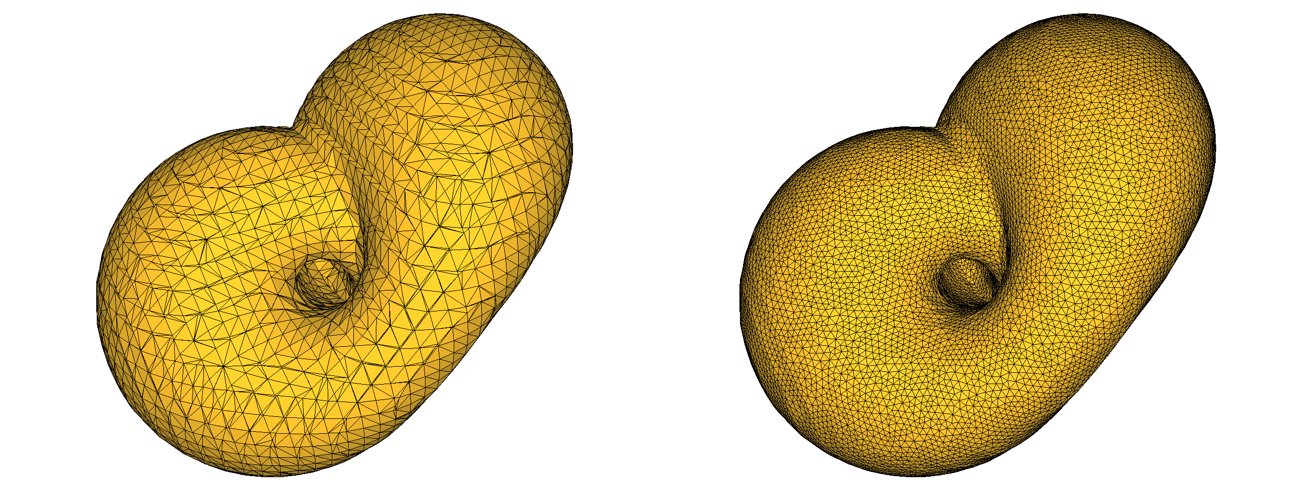
Figure 64.6 Results of the Marching Cubes algorithm, and the final result after remeshing.
The following example illustrates a basic run of the Dual Contouring algorithm, and in particular the free function to create a domain from a Cartesian grid, and the named parameters that enable (or disable) triangulation of the output, and to constrain the vertex location within the cell.
Example: Isosurfacing_3/dual_contouring.cpp
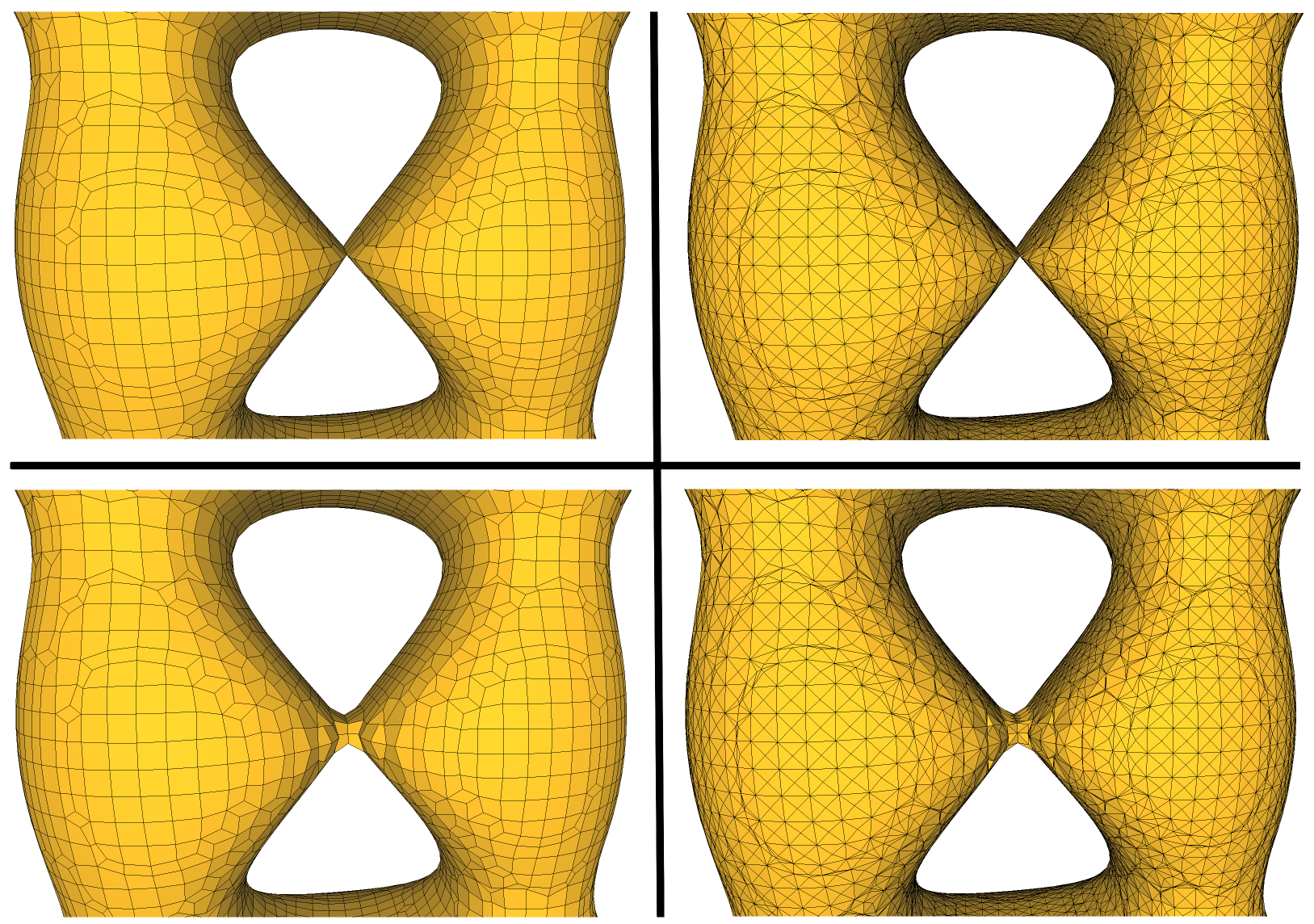
Figure 64.7 Results of the Dual Contouring algorithm: untriangulated (left column) or triangulated (right column), unconstrained vertex location (top row) or constrained vertex location (bottom row).
The following example shows the usage of Marching Cubes and Dual Contouring algorithms to extract an isosurface. The domain is implicit and describes the unit sphere by the distance to its center (set to the origin) as an implicit 3D value field.
Example: Isosurfacing_3/contouring_implicit_data.cpp
In the following example, the input data is sampled at the vertices of a grid, and interpolated.
Example: Isosurfacing_3/contouring_discrete_data.cpp
The following example shows how to load data from an Image_3, and generates an isosurface from this voxel data.
Example: Isosurfacing_3/contouring_inrimage.cpp
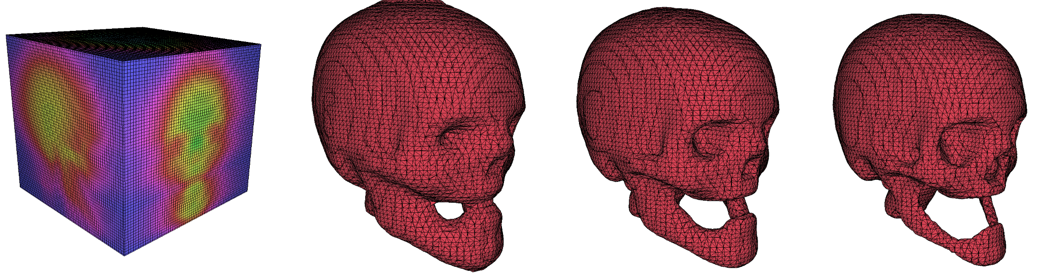
Figure 64.8 Results of the Topologically Correct Marching Cubes algorithm for different isovalues (1, 2, and 2.9) on the skull model.
The following example illustrates how to generate a mesh approximating a signed offset to an input closed surface mesh. The input mesh is stored into an AABB_tree data structure to provide fast distance queries. Via the Side_of_triangle_mesh functor, the sign of the distance field is made negative inside the mesh.
Example: Isosurfacing_3/contouring_mesh_offset.cpp
The following example shows the use of an octree as discretization instead of a Cartesian grid for both Dual Contouring and Marching Cubes. Note that in this configuration, all methods lose guarantees, and cracks can easily appear in the surface for Marching Cubes if the octree is not adapted to the surface being extracted.
Example: Isosurfacing_3/contouring_octree.cpp
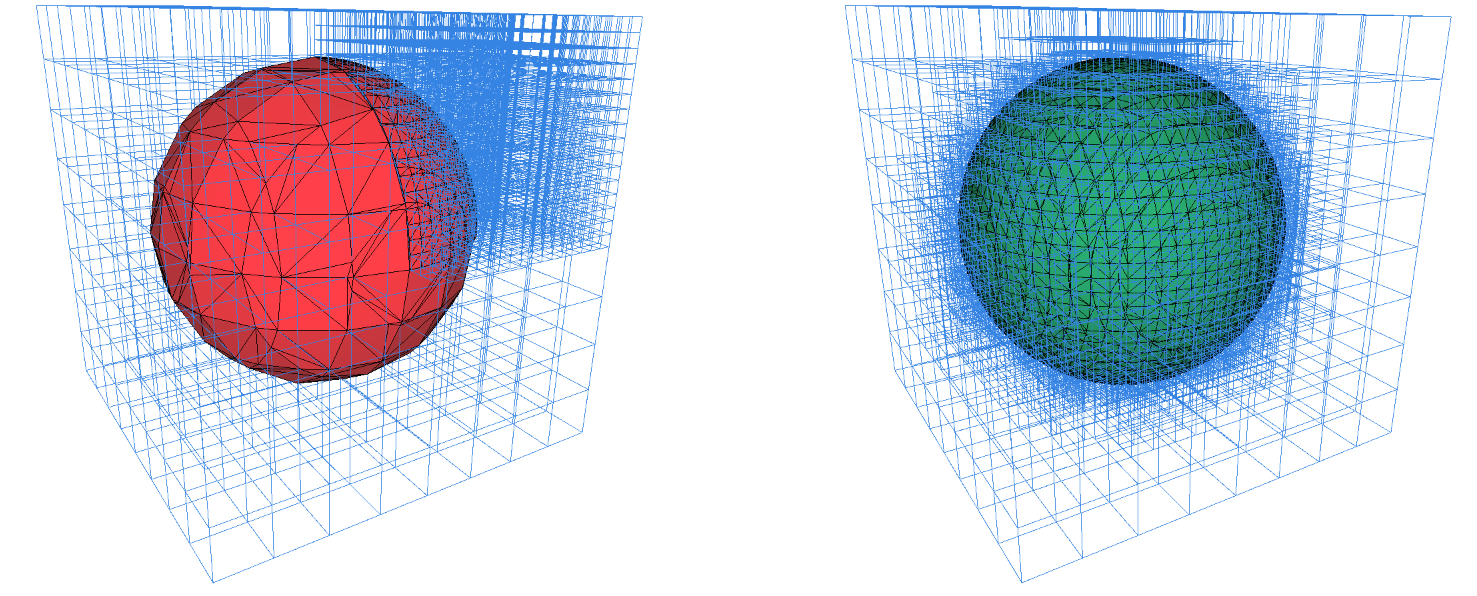
Figure 64.9 Running Marching Cubes with an octree: left, the octree (blue wireframe) has been applied arbitrary refinement in one eighth of the domain and the resulting mesh exhibits cracks (boundaries) at the regions where octree levels are discontinuous. Right, the octree was constructed to be dense around the isosurface, and the surface is manifold.
The development of this package started during the 2022 Google Summer of Code, with the contribution of Julian Stahl, mentored by Daniel Zint and Pierre Alliez, providing a first implementation of Marching Cubes, Topologically Correct Marching Cubes, and Dual Contouring. Marching Cubes tables were provided by Roberto Grosso (FAU Erlangen-Nürnberg). Mael Rouxel-Labbé worked on improving the initial Dual Contouring implementation, and on the first complete version of the package.