
|
CGAL 6.2 - Convex Decomposition of Polyhedra
|
Loading...
Searching...
No Matches
|
CGAL 6.2 - Convex Decomposition of Polyhedra
|
For many applications on non-convex polyhedra, there are efficient solutions that first decompose the polyhedron into convex pieces. As an example, the Minkowski sum of two polyhedra can be computed by decomposing both polyhedra into convex pieces, compute pairwise Minkowski sums of the convex pieces, and unite the pairwise sums.
While it is desirable to have a decomposition into a minimum number of pieces, this problem is known to be NP-hard [1]. This package offers two methods for decomposing polyhedra. The Convex Decomposition of Nef Polyhedra splits polyhedra into convex pieces with an upper bound on their number. The Approximate Convex Decomposition method offers a fast approximate decomposition of the convex hull into convex volumes. While any number of convex volumes can be generated, these convex volumes are more compact than the convex hull, but still include additional empty space than just the input polyhedron.
The method decomposes a Nef polyhedron \( N\) into \(O(r^2)\) convex pieces, where \( r\) is the number of edges that have two adjacent facets that span an angle of more than 180 degrees with respect to the interior of the polyhedron. Those edges are also called reflex edges. The bound of \(O(r^2)\) convex pieces is worst-case optimal [1].
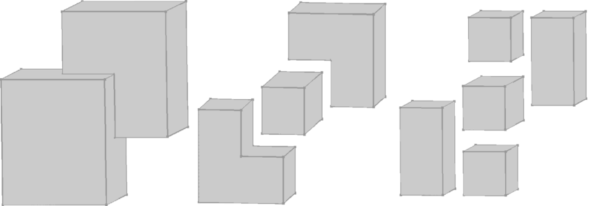
Figure 34.1 Vertical decomposition based on the insertion of vertical facets (viewed from the top). Left: Non-convex polyhedron. Middle: Non-vertical reflex edges have been resolved. Right: Vertical reflex edges have been resolved. The sub-volumes are convex.
The decomposition runs in two steps. In the first step, each non-vertical reflex edge \( e\) is resolved by insertion of vertical facets through \( e\). In the second step, the vertical reflex edges are handled in the same way. Figure 34.1 illustrates the two steps.
At the moment the implementation is restricted to the decomposition of bounded polyhedra.
An instance of Nef_polyhedron_3 represents a subdivision of the three-dimensional space into vertices, edges, facets, and volumes. Some of these items form the polyhedron (selected), while others represent the outer volume or holes within the polyhedron (unselected). As an example, the unit cube is the point set \( [0,1]^3\). The smallest subdivision that represents the unit cube has 8 vertices, 12 edges, 6 facets, and 2 volumes. The volumes enclosed by the vertices, edges, and facets is the interior of the cube and therefore selected. The volume outside the cube does not belong to it and is therefore unselected. The vertices, edges, and facets - also denoted as boundary items - are needed to separate the two volumes, but are also useful for representing topological properties. In case of the (closed) unit cube the boundary items are part of the polyhedron and therefore selected, but in case of the open unit cube \( [0,1)^3\) they are unselected. Each item has its own selection mark, which allows the correct representation of Nef polyhedra, which are closed under Boolean and topological operations. Details can be found in Chapter 3D Boolean Operations on Nef Polyhedra.
Usually, an instance of Nef_polyhedron_3 does not contain any redundant items. However, the function convex_decomposition_3() subdivides selected volumes of a given Nef_polyhedron_3 by selected facets. These additional facets are therefore redundant, i.e., their insertion alters the representation of the polyhedron, but not the polyhedron itself.
When convex_decomposition_3() resolved all reflex edges, the selected sub-volumes have become convex. Each of them is represented by a separate volume item and can therefore be traversed separately as described in Section Exploring Shells. Another possibility of accessing the convex pieces is to convert them into separate Nef polyhedra, as illustrated by the example code given below.
Note that due to the restriction to bounded polyhedra, the use of extended kernels is unnecessary and expensive. Therefore the use of extended kernels in the convex decomposition is not supported.
This example shows the usage of CGAL::convex_decomposition_3(Nef_polyhedron_3&) to decompose a Nef polyhedron into convex parts.
File Convex_decomposition_3/list_of_convex_parts.cpp
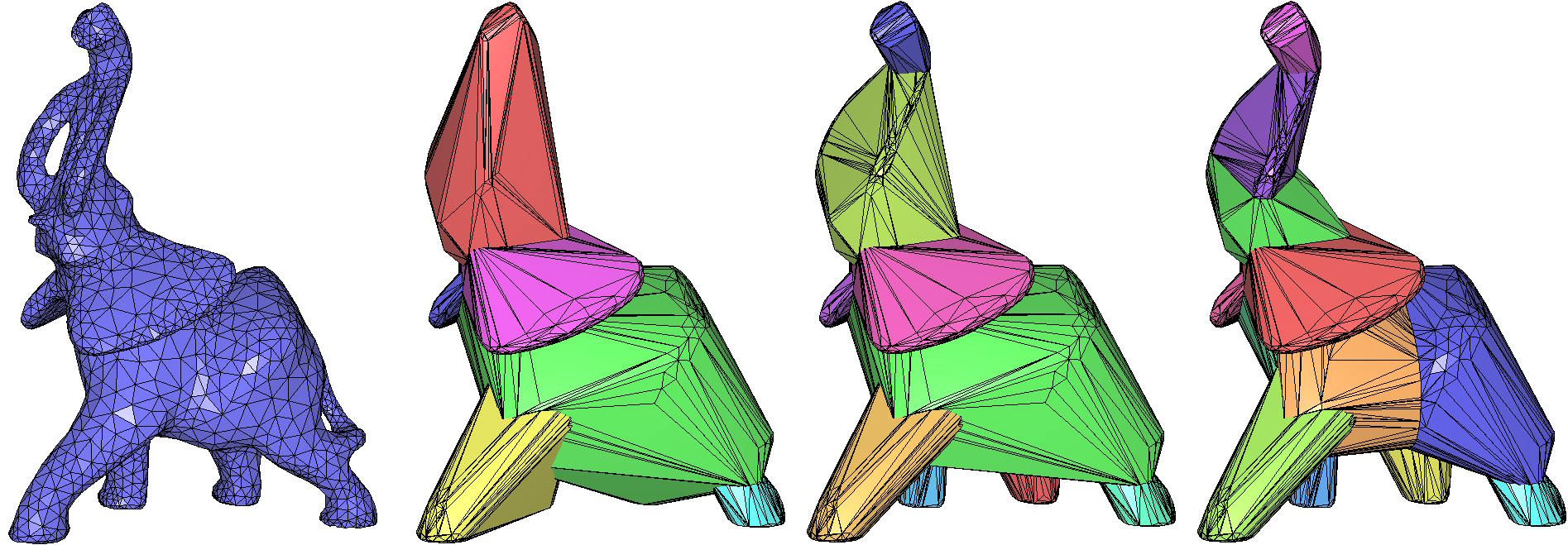
Figure 34.2 Approximate convex decomposition of the elephant.off model.
From left to right: input mesh, 6, 9, and 12 convex volumes
The H-VACD method [2], "Hierarchical volumetric approximate convex decomposition", computes a set of convex volumes that fit the polyhedron. Contrary to the decomposition of the polyhedron into convex parts, the convex volumes cover the polyhedron, but also include additional volume outside of it. A sufficiently tight enclosure of the polyhedron by several convex volumes allows fast intersection calculation and collision detection among polyhedra while offering a non-hierarchical approach and may thus be easier to use in a parallel setting. The resulting set of convex volumes minimizes the volume between their union and the polyhedron while fully including the input polyhedron. While the optimal solution with n convex hulls that cover the polyhedron with the smallest additional volume remains NP-hard, this method provides a fast error-driven approximation.
The algorithm computes a set of convex volumes \( C=\{C_i\) with \( i \in[0..n-1]\} \) that cover the input polyhedron while minimizing the additional covered volume:
\begin{equation} \arg \min_C d(\bigcup_{C_i \in C} C_i, P) \\ \end{equation}
\begin{equation} d(A, B) = |A| - |B| \end{equation}
Where \(|A|\) is the volume of A, P is the input polyhedron and \(C_i\) are convex volumes. The convex volumes \(C_i\) are may slightly overlap and their union contain the input polyhedron \( P \subset \bigcup_{C_i \in C} \).
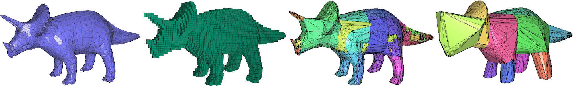
Figure 34.3 Approximate convex decomposition pipeline.
From left to right: 1. input mesh 2. voxel grid 3. convex volumes after error-driven splitting 4. final convex volumes after merging
The method employs a top-down splitting phase followed by a bottom-up merging to achieve the target number of convex volumes. The splitting phase aims at decomposing the input mesh into smaller mostly convex parts. Each part of the input mesh is approximated with its convex hull. In a hierarchical manner, each part of the mesh is split into two parts when its convexity is low. The convexity is measured by the volume difference of the part and its convex hull. Splitting a part into two can be done by simply cutting the longest side of the bounding box in half. A better choice is often found by searching the longest side of the bounding box for a concave spot. However, it comes with a higher computational cost. The hierarchical splitting stops when either the convexity is sufficiently high or the maximum depth is reached. The volume calculation, convex hull computation and the concavity search is accelerated by a voxel grid. The grid is prepared before the splitting phase and voxel cells overlapping with triangles are labeled as surface. The remaining voxels are labeled as outside or inside by flood fill, in case the input mesh is closed, or by axis-aligned ray shooting, i.e., along x, y and z-axes in positive and negative directions. A voxel is only labeled as inside if at least 3 faces facing away from the voxel have been hit and no face facing towards the voxel. The convex hulls are calculated from voxel corners. Thus, a mesh with a high resolution is less penalized by its number of vertices. The splitting phase typically results in a number of convex volumes larger than targeted.
To optionally improve the fit of the convex volumes, they can be refitted to the mesh before starting the second phase. The second phase employs a bottom-up merging that reduces the number of convex volumes to the targeted number while aiming at maintaining a low volume difference between convex volumes and the input mesh. The greedy merging maintains a priority queue to incrementally merge the pair of convex volumes with the smallest increase of volume difference.
The splitting phase is not limited by the chosen maximum_number_of_convex_volumes, because a splitting into a larger number of more convex parts with a subsequent merging leads to better results.
Due to the hierarchical splitting using planes, it is possible that a convex volume is degenerated. In the merging phase, these degenerated convex volumes are merged with a high priority. However, it is possible that the output of the method still contains degenerated convex volumes. This is especially the case, when a large maximum_number_of_convex_volumes is chosen while using a limited maximum_depth.
Several parameters of the algorithm impact the quality of the result as well as the running time.
maximum_number_of_convex_volumes: The maximum number of convex volumes output by the method. The actual number may be lower for mostly convex input meshes, e.g., a sphere. The impact on the running time is rather low. The default is 16.maximum_depth: The maximum depth for the hierarchical splitting phase. For complex meshes, a higher maximum depth is required to split small concavities into convex parts. The choice of maximum_depth has a larger impact on the running time. The default is 10.refitting: The convex hulls can be refitted after the splitting phase to more tightly enclose the input mesh. It increases the running time, but significantly reduces the overhead volume included by the computed convex volumes. It is enabled by default.maximum_number_of_voxels: This parameter controls the resolution of the voxel grid used for speed-up. Larger numbers result in a higher memory footprint and a higher running time. A small number also limits the maximum_depth. The voxel grid is isotropic and the longest axis of the bounding box will be split into a number of voxels equal to the cubic root of maximum_number_of_voxels. The default value is 1.000.000.volume_error: The splitting of a convex volume into smaller parts is controlled by the volume_error which provides the tolerance for difference in volume. The difference is calculated by \( (|C_i| - |P_i|) / |P_i|\). The default value is 0.01. Thus, if a convex volume has 1 percent more volume that the part of the input mesh it approximates, it will be further divided.split_at_concavity: The splitting can be either performed after searching a concavity on the longest side of the bounding box or simply by splitting the longest side of the bounding box in half. The default value is true, i.e., splitting at the concavity.The method is demonstrated on a few models:
| Data set | Faces | Volume | Convex hull volume | Overhead |
|---|---|---|---|---|
| Camel | 19.536 | 0.0468 | 0.15541 | 2.32388 |
| Elephant | 5.558 | 0.0462 | 0.12987 | 1.81087 |
| Triceratops | 5.660 | 136.732 | 336.925 | 1.46412 |
| Knot2 | 11.520 | 0.0488 | 0.19141 | 2.92334 |
The overhead is the convex hull volume divided by the volume of the mesh. If not mentioned otherwise, all tests used a volume error of 0.01, a maximum depth of 10, 1 million voxels and split at the concavity.
Impact of varying the number of generated convex volumes with splitting at the concavity and refitting to the convex hull of the input mesh on volume overhead:
| Data set | Split location | Refitting | 4 volumes | 6 volumes | 8 volumes | 10 volumes | 12 volumes | Running time |
|---|---|---|---|---|---|---|---|---|
| Camel | Concavity | + | 0.6951 | 0.4316 | 0.3016 | 0.2514 | 0.1955 | 2.22s |
| Camel | Concavity | - | 0.9932 | 0.7482 | 0.6174 | 0.5507 | 0.5261 | 1.20s |
| Camel | Mid | + | 0.7994 | 0.5589 | 0.3928 | 0.3211 | 0.2266 | 2.58s |
| Camel | Mid | - | 1.0875 | 0.9280 | 0.8394 | 0.6801 | 0.5529 | 1.29s |
| Elephant | Concavity | + | 0.7897 | 0.6505 | 0.4973 | 0.3986 | 0.3299 | 1.16s |
| Elephant | Concavity | - | 1.2140 | 1.0028 | 0.8071 | 0.7290 | 0.6870 | 0.98s |
| Elephant | Mid | + | 0.7448 | 0.5692 | 0.4453 | 0.3844 | 0.2912 | 1.99s |
| Elephant | Mid | - | 1.2075 | 1.0410 | 0.8247 | 0.6779 | 0.6263 | 1.45s |
| Triceratops | Concavity | + | 0.5952 | 0.3978 | 0.3548 | 0.2385 | 0.2057 | 1.03s |
| Triceratops | Concavity | - | 1.0073 | 0.7490 | 0.7035 | 0.5966 | 0.5429 | 0.59s |
| Triceratops | Mid | + | 0.7149 | 0.4380 | 0.3984 | 0.2801 | 0.2303 | 1.53s |
| Triceratops | Mid | - | 1.0470 | 0.8990 | 0.6749 | 0.5803 | 0.5237 | 0.91s |
| Knot2 | Concavity | + | 1.2721 | 0.9538 | 0.6395 | 0.4748 | 0.4040 | 1.95s |
| Knot2 | Concavity | - | 1.7901 | 1.4242 | 1.1538 | 0.9394 | 0.8496 | 1.49s |
| Knot2 | Mid | + | 1.2451 | 0.9286 | 0.6178 | 0.4373 | 0.3558 | 2.08s |
| Knot2 | Mid | - | 1.7143 | 1.3477 | 1.0436 | 0.9030 | 0.7910 | 1.78s |
The columns for the different number of volumes indicate the overhead of the union of the convex volumes compared to the volume of the mesh. Note that the convex volumes may overlap, thus the volume of their union may be lower than the sum of volumes. Although searching the voxel grid for the concavity takes additional computational time, it is compensated by fewer splits.
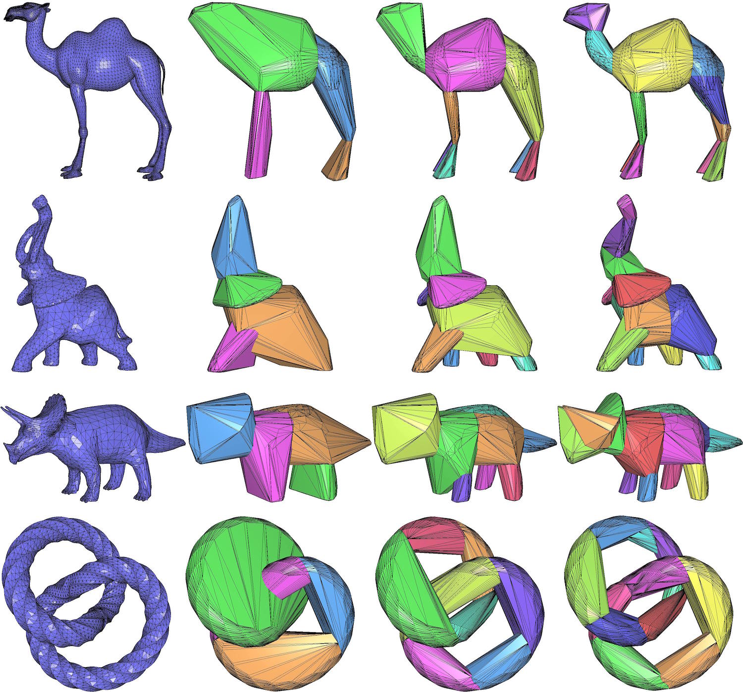
Figure 34.4 Approximate convex decomposition results.
From left to right: input mesh, 4, 8, and 12 convex volumes
The example shows the approximate convex decomposition of the knot2.off mesh into 9 convex volumes that are saved as off files.
File Convex_decomposition_3/approximate_convex_decomposition.cpp
This package was created by Peter Hachenberger with the CGAL::convex_decomposition_3() method. In 2025, it has been extended by Sven Oesau with the CGAL::approximate_convex_decomposition() method.