
|
CGAL 6.2 - 2D Alpha Wrapping
|
Loading...
Searching...
No Matches
|
CGAL 6.2 - 2D Alpha Wrapping
|
Note: a three-dimensional version of this package is also available: 3D Alpha Wrapping.
Various tasks in geometric modeling and processing require 2D objects represented as valid polygons, where "valid" refers to polygons that are closed, intersection-free (simple), orientable, and 1-manifold. Such representations offer well-defined notions of interior/exterior and geodesic neighborhoods.
2D data are usually acquired through measurements, possibly followed by reconstruction, designed by humans, or generated through imperfect automated processes. As a result, they can exhibit a wide variety of defects including gaps, missing data, self-intersections, degeneracies such as zero-area structures, and non-manifold features.
Given the large repertoire of possible defects, many methods and data structures have been proposed to repair specific defects (see for example the package 2D Polygon Repair), usually with the goal of guaranteeing specific properties in the repaired 2D model. Reliably repairing all types of defects is an ill-posed problem as many valid solutions exist for a given 2D model with defects. In addition, the input model can be overly complex with unnecessary geometric details, spurious topological structures, nonessential inner components, or excessively fine discretizations. For applications such as collision avoidance, path planning, or simulation, getting an approximation (i.e., a silhouette) of the input can be more relevant than repairing it. Approximation herein refers to an approach capable of filtering out inner structures, fine details and cavities, as well as wrapping the input within a user-defined offset margin.
Given an input 2D geometry, we address the problem of computing a conservative approximation, where conservative means that the output is guaranteed to strictly enclose the input. We seek unconditional robustness in the sense that the output polygon should be valid (oriented, 1-manifold, and without self-intersections), even for raw input with many defects and degeneracies. The default input is a soup of 2D segments, but the generic interface leaves the door open to other types of finite 2D primitives such as point sets.
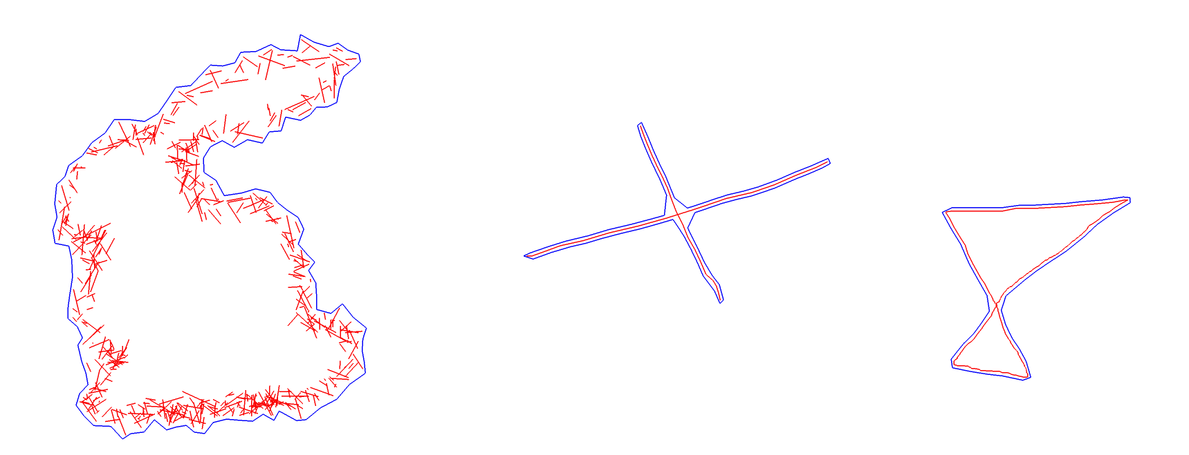
Figure 60.1 (Left) Shrink-wrapping output from a segment soup with many intersections and gaps. (Center & Right) Possible input degeneracies: non-manifold vertices and zero-area structures. The algorithm handles these cases by wrapping an offset of the input.
Many approaches have been devised to enclose a 2D model within a volume, featuring different balances between the runtime and quality (i.e., tightness) of the approximation. Within the simplest cases, an axis-aligned or oriented bounding box clearly satisfies some desired properties; however, the approximation error is uncontrollable and often very large. Computing the convex hull of the input also matches some of the desired properties and improves the quality of the result, albeit at the price of increasing the runtime. However, the approximation remains crude, especially in the case of several components.
The convex hull is, in fact, a special case of alpha shapes (Chapter_2D_Alpha_Shapes). Mathematically, the alpha shape is a subcomplex of the Delaunay triangulation, with simplicies being part of the complex depending on the size of their minimal (empty) Delaunay ball. Intuitively, constructing 2D alpha shapes can be thought of as carving 2D space with an empty ball of user-defined radius alpha. Alpha shapes yield provable, good piecewise-linear approximations of a shape [1], but are defined on point sets, whereas we wish to deal with more general input data, such as segment soups. Even after sampling the segment soup, alpha shapes do not guarantee to be conservative for any alpha. Finally, inner structures are also carved within the volumes, instead of being filtered out.
Inspired by alpha shapes, we replace the above notion of carving by shrink-wrapping: we iteratively construct a subcomplex of a 2D Delaunay triangulation by starting from a simple 2D Delaunay triangulation enclosing the input, and then iteratively removing eligible triangles that lie on the boundary of the complex. In addition, the underlying triangulation—and thus the complex incidentally—is refined as shrinking proceeds. Thus, instead of carving from the convex hull of the input data as in alpha shapes, we construct an entirely new polygon through a Delaunay refinement-like algorithm. The refinement algorithm inserts Steiner points on the boundary of an offset volume, defined as a level set of the unsigned distance field to the input.
This process both prevents the creation of inner structures within the output and avoids superfluous computations. In addition, detaching our wrap construction from the geometry and discretization of the input has several advantages: (1) the underlying data is not restricted to a specific format (polygon soups, segment soups, point sets, etc.) as all that is required is answering three basic geometric queries: (a) the distance between a point and the input, (b) the projection of a query point onto the input, (c) an intersection test between a triangle and the input, and (2) The user has more freedom to trade tightness to the input for final polgyon complexity, as constructing a conservative approximation on a large offset of the input requires fewer polygon edges.
Initialization. The algorithm is initialized by inserting the four corner vertices of a loose bounding box into a 2D Delaunay triangulation. In the 2D Delaunay triangulation of CGAL, all edges are adjacent to two triangle faces. Each edge of the boundary of the Delaunay triangulation, which coincides with one edge of the convex hull of the triangulation vertices, is adjacent to a so-called infinite triangle face, an abstract face connected to the so-called infinite vertex to ensure the aforementioned double-edge adjacency. Initially, all infinite faces are tagged as outside, and all finite triangle faces are tagged as inside.
Shrink-wrapping. The shrink-wrapping algorithm proceeds by traversing the faces of the Delaunay triangulation from outside to inside, flood-filling from one face to its adjacent face, and tagging the adjacent face as outside whenever possible (the term "possible" is specified later). Flood filling is implemented via a priority queue of Delaunay triangle edges representing the traversal between the two adjacent faces of the edge, from outside to inside. These edges are referred to as gates in the following.
Given an outside face and its adjacent inside face, the common edge (i.e., a gate) is said to be alpha-traversable if its circumradius is larger than the user-defined parameter alpha, where circumradius refers to the radius of the relating segment's Delaunay ball. Intuitively, cavities smaller than alpha are not accessible as their gates are not alpha-traversable.
Initialized by the alpha-traversable gates on the convex hull, the priority queue contains only alpha-traversable gates and is sorted by decreasing order of the circumradius of the gate. Traversal can be seen as a continuous process that advances along dual Voronoi edges of the gates, with a pencil of empty balls circumscribing the gate.
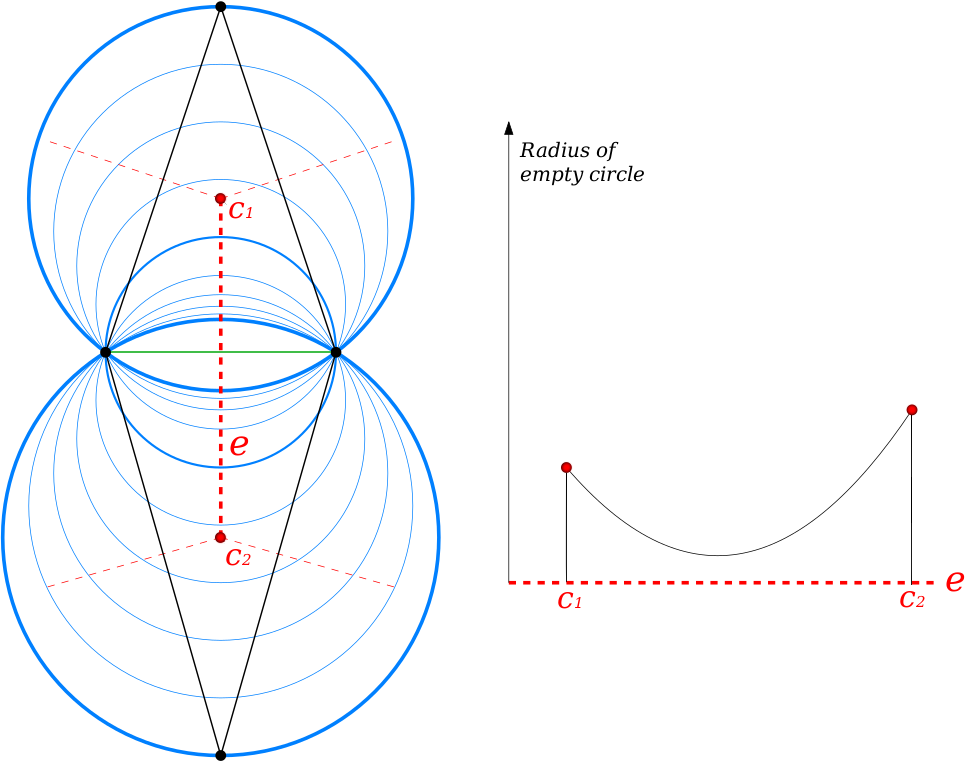
Figure 60.2 (Left) Pencil of empty circles (blue) circumscribing a Delaunay edge (green) in a 2D Delaunay triangulation (black). From the top triangle circumcenter c1 to the bottom triangle circumcenter c2, the dual Voronoi edge denoted by e (doted red) is the trace of centers of the largest circles that are empty of Delaunay vertex. (Right) The graph corresponding to the left example. The x-axis corresponds to the position of empty circle centers located on the Voronoi edge e, from c1 to c2. The y-axis is the radius value of the corresponding empty circles. In this case, the minimum radius of this pencil of empty circle is located at the midpoint of the green Delaunay edge. In our algorithm, a gate (green Delaunay edge) is said to be not alpha-traversable when the minimum radius of the pencil of empty circle is smaller than alpha.
When traversing from an outside face \( f_o \) to an inside face \( f_i \) through an alpha-traversable edge \( e \), two criteria are tested to prevent the wrapping process from colliding with the input:
(1) We check for an intersection between the dual Voronoi edge of \( e \), i.e. the segment between the circumcenters of the two incident faces, and the offset surface, defined as the level set of unsigned isosurface to the input. If one or several intersections exists, the first intersection point, along the dual Voronoi edge oriented from outside to inside is inserted into the triangulation as a Steiner point.
(2) If the dual Voronoi edge does not intersect the offset surface but the neighboring face \( f_i \) intersects the input, we compute the projection of the circumcenter of \( f_i \) onto the offset surface, and insert it into the triangulation as a Steiner point (which destroys \( f_i \)).
After each of the above Steiner point insertions, all new incident faces are tagged as inside, and the newly alpha-traversable gates are pushed into the priority queue.
If none of the above two criteria are met, the neighboring face \( f_i \) is traversed and tagged as outside. Alpha-Traversable edges of \( f_i \) that are separating inside from outside faces are pushed as new gates into the priority queue.
Once the queue empties—a process that is guaranteed as edges (and their circumradii) become smaller due to the insertion of new Steiner points—the construction phase terminates. The output (multi)polygon is extracted from the Delaunay triangulation as the set of edges separating inside from outside faces.
The figure below depicts the steps of the algorithm.
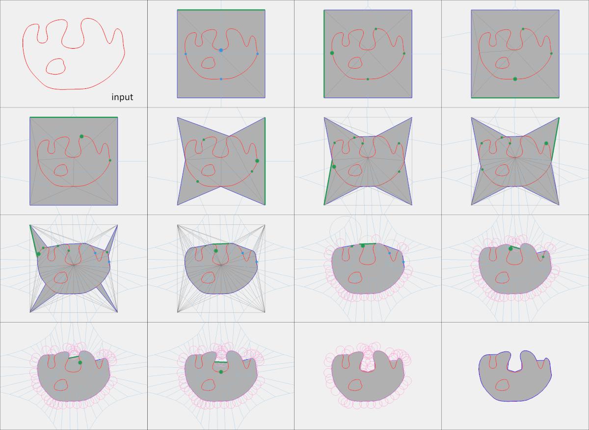
Figure 60.3 Steps of the shrink-wrapping algorithm in 2D. The algorithm is initialized by inserting the corners of the loose bounding box of the input (red) into a Delaunay triangulation, and all finite triangles are tagged inside (grey). The current gate (green edge) popped out from the queue is alpha-traversable. The triangle adjacent to the gate is tagged outside when it does not intersect the input, and new alpha-traversable gates are pushed to the queue. When the adjacent triangle intersects the input, a new Steiner point (large green disc) is computed and inserted into the triangulation, all neighboring triangles are tagged inside, new alpha-traversable gates are pushed to the queue, and traversal is resumed. Grey edges depict the Delaunay triangulation. Blue edges depict the Voronoi diagram. Pink circles depict the empty circle of radius alpha. The output edges (dark blue) separate inside from outside triangles.
The algorithm is proven to terminate and to produce a set of 1-manifold, simple polygons that strictly enclose the input data. The key element to the proof is that we wrap from outside to inside and never allow a face that intersects the input to be flagged inside. Furthermore, both criteria that lead to refinement of the triangulation insert Steiner points that are guaranteed to break the faces in need of refinement and reduce the neighbor edges' circumradii.
Because the main refinement criterion is the insertion of an intersection between a dual Voronoi edge and an offset of the input, or the projection of a Voronoi vertex onto the offset of the input, the algorithm has similarities to popular meshing algorithms based on Delaunay filtering and refinement (see Chapter_3D_Mesh_Generation).
Our algorithm takes as input a set of segments in 2D, provided either as a segment soup or as a set of polygons, and two user-defined scalar parameters: the alpha and the offset values. It proceeds by shrink-wrapping and refining a 2D Delaunay triangulation starting from a loose bounding box of the input. The parameter alpha refers to the size of cavities or holes that cannot be traversed during wrapping, and hence to the final level of detail, as alpha acts like a sizing field in a common Delaunay refinement algorithm (Chapter_3D_Mesh_Generation). The parameter offset refers to the distance between the vertices of the refined triangulation and the input, so that a large offset translates into a loose enclosing of the input. This second parameter offers a means to control the trade-off between tightness and complexity.
The main entry point of the component is the global function CGAL::alpha_wrap_2() that generates the alpha wrap; this function takes as input a point set, a polyline soup, or a polygon soup. There is no prerequisite on the input connectivity so that it can take inputs with islands, self-intersections, or overlaps, as well as combinatorial or geometrical degeneracies.
The underlying traits class must be a model of the Kernel concept. It should use a floating point number type as inexactness is inherent to the algorithm since there is no closed form description of new vertices on the offset surface.
The output is a multi polygon, i.e., a set of polygons, whose type is chosen by the user, under the constraint that it must be a model of the MultiPolygonWithHoles_2 concept.
The two parameters of the algorithm impact both the level of detail and complexity of the output wrap.
The main parameter, alpha, controls whether a Delaunay edge is traversable during shrink-wrapping. Alpha's main purpose is to control the size of the empty balls used during wrapping, and thus to determine which features will appear in the output: indeed, a edge is alpha-traversable if its circumradius is larger than alpha; hence, the algorithm can only shrink-wrap through straits or holes with diameters larger than alpha. A second, less direct consequence is that as long as a edge has a circumradius larger than alpha, the incident inside face will be visited and possibly refined. Therefore, when the algorithm terminates, all edges have a circumradius smaller than alpha. This parameter thus also behaves like a sizing criterion on the edges of the output.
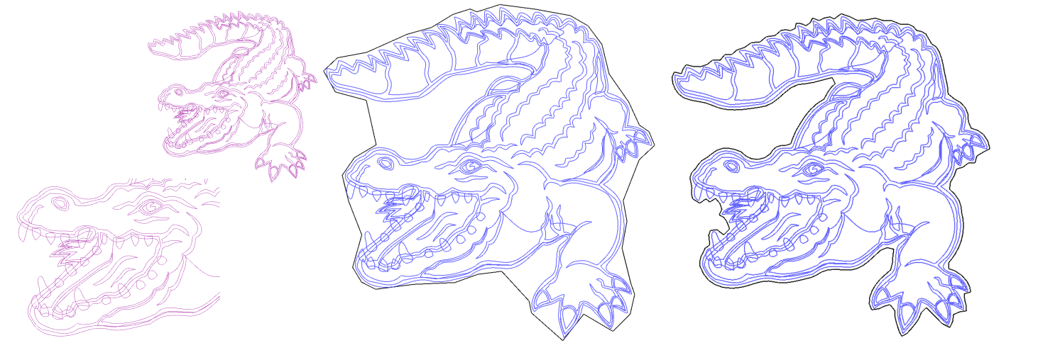
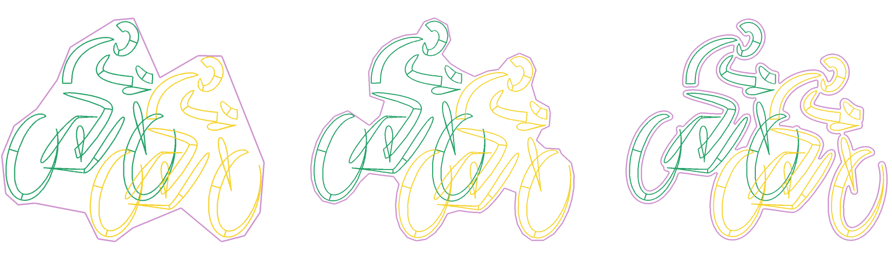
Figure 60.4 Impact of the alpha parameter on the output. (Left) The input segment soup, generated from an SVG file. The input has many self-intersections, non-manifold vertices, superfluous geometric details and spurious topological structures. (Middle & Right) This component approximates the input conservatively and produces valid polygons with different complexity and fidelity to the input, depending on the alpha parameter. The smaller the alpha, the deeper the shrink-wrapping process will enter cavities. The alpha parameter is decreasing from left to right, to respectively 1/50, 1/100 and 1/300 of the longest diagonal of the input bounding box. A large alpha will produce an output less complex but less faithful to the input.
The second parameter, the offset distance, controls the distance from the input and thus the definition of the offset isosurface onto which the vertices of the output polygon are located. This parameter controls the tightness of the result, which has, in turn, a few consequences. Firstly, locating vertices away from the input enables the algorithm to generate a less complex result, especially in convex areas. A trivial example of this behavior would be a very dense circle-shaped polygon, for which an as-tight-as-possible envelope would also need to be very dense. Secondly, the farther the isosurface is from the input, the more new points are inserted through the first criterion (i.e., through intersection with dual Voronoi edge, see Section Algorithm); thus, the quality of the output improves in terms of angles of the triangle elements. Finally, and depending on the value of the alpha parameter, a large offset can also offer defeaturing capabilities. However, using a small offset parameter will tend to better preserve sharp features as projection Steiner points tend to project onto convex sharp features.
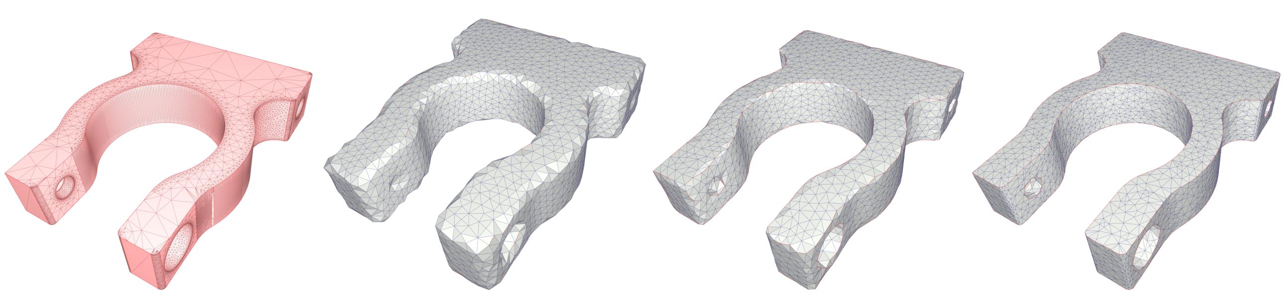
Figure 60.5 [TO BE UPDATED] Impact of the offset parameter on the output. (Left) Input mesh generated by meshing a NURBS CAD model in parameter space. (Right) The smaller the offset, the closest sample points are to the input. The offset parameter is decreasing from left to right, to respectively 1/50, 1/200 and 1/1000 of the longest diagonal of the input bounding box. The alpha parameter is equal to 1/50 of the longest diagonal of the input bounding box for all level of details. A larger offset will produce an output less complex with better triangle quality. However, the sharp features (red edges) are well-preserved when the offset parameter is small.
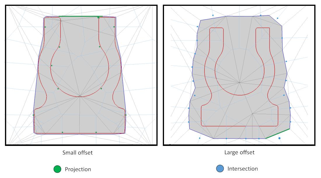
Figure 60.6 Steiner points. The projection Steiner points (green) are computed by projecting the triangle circumcenter onto the offset. The intersection Steiner points (blue) are computed as the first intersection point between the Voronoi edge and the offset. (Left) When the offset parameter is small, the algorithm produces more projection Steiner points, which tends to improve the preservation of convex sharp features. (Right) When the offset parameter is large, the algorithm produces more intersection Steiner points.
By default, we recommend to set the offset parameter to a small fraction of alpha, such that alpha becomes the main parameter that controls the final level of detail.
The image below illustrates the impact of both parameters.
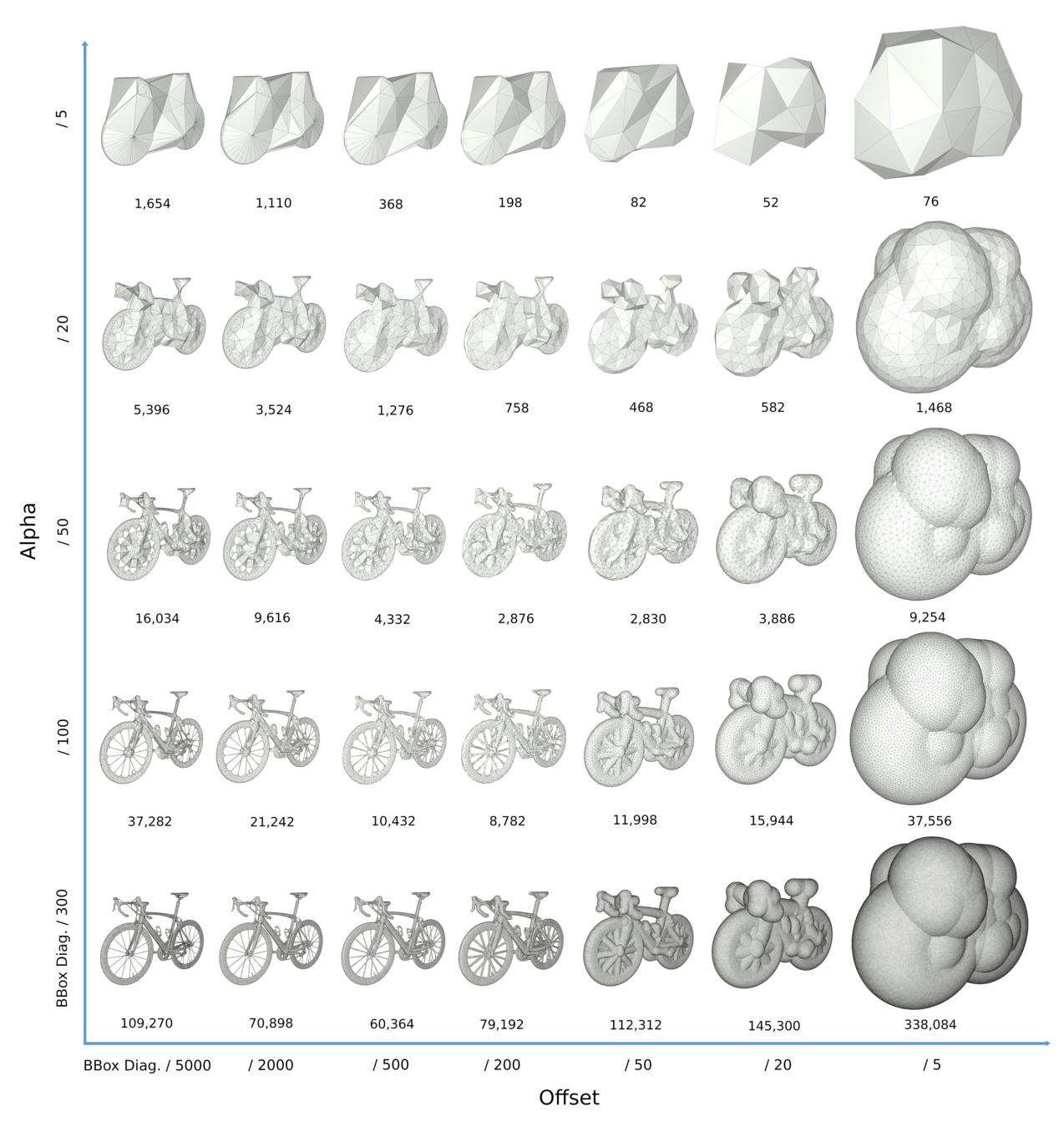
Figure 60.7 [UPDATE] Different alpha and offset values on the bike model (533,000 triangles). The x-axis represents the offset value equal to 1/5000, 1/2000, 1/500, 1/200, 1/50, 1/20 and 1/5 of the longest diagonal of the input bounding box, from left to right. The y-axis represents the alpha value equal to 1/300, 1/100, 1/50, 1/20 and 1/5 of the longest diagonal of the input bounding box, from bottom to top. The numbers below each level of detail represents their number of triangles. Depending on the alpha value, an offset too small or too large will produce outputs with higher complexity. For each alpha, the models with lower complexity can be used as a scale-space representations for collision detection, from near to far distances.
The offset parameter is crucial to our approach because it guarantees that the output is a set of 1-manifold, simple polygons. Indeed, and even when the input is a zero-area structure such as a single segment, the output wrap is a thin domain enclosing the said segment Figure 60.1.
Users should keep in mind that the wrapping algorithm performs with an the unsigned distance field, and has no means of determining whether it is acting on both sides of a same input segment. It will thus produce two-sided wraps in the case of holes in the input and values of alpha smaller than the size of the holes.
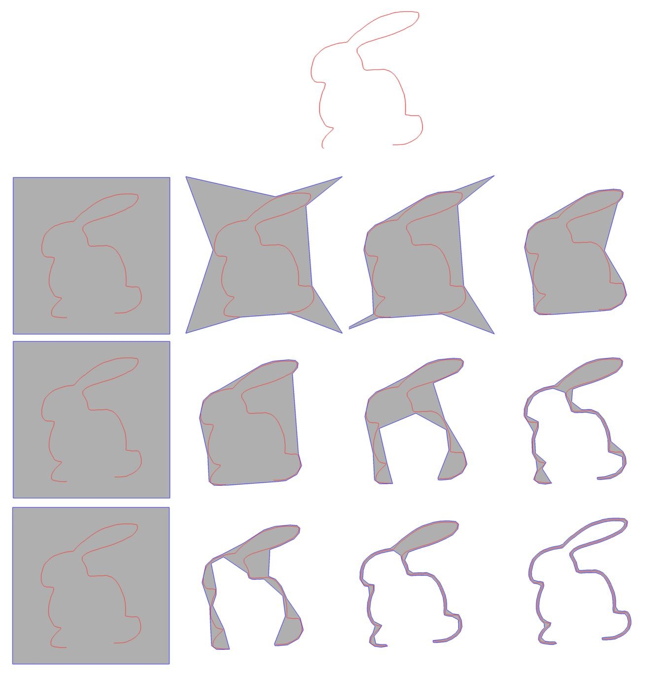
Figure 60.8 Wrapping a Bunny in 2D, with decreasing values for alpha. When alpha is small enough with respect the diameter of the holes, the algorithm generates a two-sided wrap.
The following example illustrates how to construct the wrap of a soup of 2D segments. Alpha is set to 1/20 of the bounding box's longest diagonal edge length, and offset set to 1/30 of alpha (i.e., 1/600 of the bounding box diagonal edge length).
File Alpha_wrap_2/polyline_wrap_2.cpp
For polygons, we use multipolygons to represent input sets of polygons (possibly with holes). The following example uses the WKT file format to read such input and wrap it. Note the possible usage of the 2D Polygon Repair package if a pre-emptive repair of the polygons is desired.
File Alpha_wrap_2/polygon_wrap_2.cpp
Finally, the following example demonstrates how to wrap a 2D point set constructed from the projection of an input 3D point cloud.
File Alpha_wrap_2/point_set_wrap_2.cpp