Introduction
This CGAL component implements the kinetic space partition proposed by Bauchet et. al [1]. It takes as input a set of convex polygons and partitions the bounding box of the input into polyhedra, where each polyhedron and its facets are convex. Input polygons that are coplanar up to a small tolerance share a support plane and expand separately. Pieces of several coplanar polygons that initially lie in the same face of the arrangement of intersection lines within their plane are merged into their convex hull, see CGAL::Kinetic_space_partition_3::insert(). Each facet of the partition is part of the input polygons or an extension of them.
The kinetic partition homogeneously expands each input polygon along its support plane until collisions occur between them. At each collision, their expansion may stop, they may restrict the propagation along an intersection line between two support planes or they may continue beyond the intersection line. The polygons are split at the beginning of the kinetic simulation and at each collision along the intersection line to be intersection-free.
Whether a polygon is expanded beyond an intersection with another polygon, depends on the user specified k parameter. Choosing k = 1 will cause the expansion of polygons to locally stop at the first intersection with another polygon and choosing k equal to the number of input polygons will lead to a full expansion of each polygon to the bounding box.
Algorithm
The first step of the method creates a plane arrangement between the support planes of the input polygons. The computation of a plane arrangement has \(O(n^3)\). To speed up the computation the input data can be decomposed into separate kinetic partitions using an octree. The decomposition limits the expansion of an input polygon to octree nodes it initially intersects. The usage of an octree significantly speeds up the creation of the kinetic partition. However, it adds facets to the partition which originate from the octree and do not belong to an input polygon. The kinetic partitions of the octree nodes are computed independently of each other and are merged into a single conformal partition afterwards. Hence, the octree nodes can be processed in parallel, see Section Computing a Partition. The plane arrangement contains all points and lines of the intersections between the support planes and the bounding box. For each support plane, all intersections with the bounding box and other support planes are given by lines, edges and vertices of the arrangement. The kinetic partition created in the second step is a subset of faces of the arrangement depending on the k parameter.
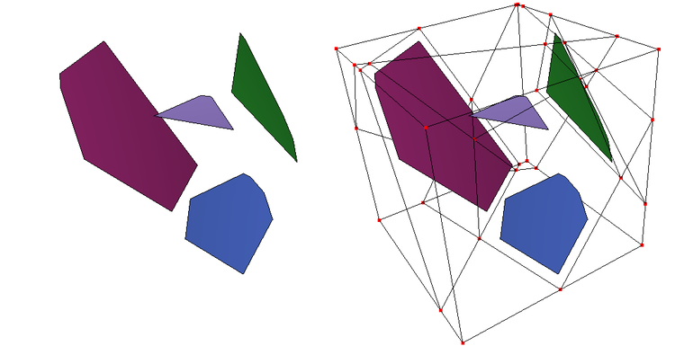
Figure 74.1 Plane arrangement.
Left: 4 convex polygons as input. Right: plane arrangement and bounding box together with input.
The kinetic partition for a chosen k is obtained by propagating each polygon within its support plane. As intersections with other polygons can only occur at the known edges in the plane arrangement, the 3D collision problem can be solved as separate 2D polygon edge collisions.
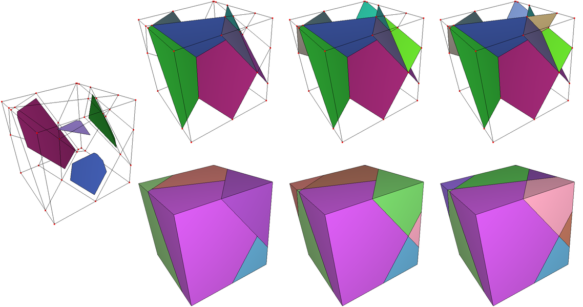
Figure 74.2 Impact of k parameter on partition.
Left: Arrangement with 4 input polygons. Right: three columns with propagated polygons on top and volumes of kinetic partition on bottom for k = 1, k = 2 and k = 3 from left to right with 5, 8 and 12 created volumes respectively.
Parameters
The algorithm has five parameters:
- k: unsigned int
The main parameter of this method is k, the maximum number of intersections that can occur for a polygon before its expansion stops. The initial intersections of the original input polygons are not considered. Thus increasing the k leads to a higher complexity of the partitioning, i.e., a higher number of facets and a higher number of volumes. For a certain k the partition can be considered to be complete and an increase in k will not further increase the complexity of the partition. A typical choice of k is in the range of 1 to 3. - reorient_bbox: boolean
The default bounding box of the partition is axis-aligned. Setting reorient_bbox to true aligns the x-axis of the bounding box with the direction of the largest variation in horizontal direction of the input data while maintaining the z-axis. - bbox_dilation_ratio: FT
By default, the size of the bounding box of the input data is increased by 10% to avoid that input polygons are coplanar with the sides of the bounding box. - max_octree_node_size: unsigned int
A kinetic partition is split into 8 subpartitions using an octree if the number of intersecting polygons is larger than specified. The default value is 40 polygons. - max_octree_depth: unsigned int
Limits the maximum depth of the octree decomposition. A limitation is necessary as arbitrary dense polygon configurations exist, e.g., a star. The default value is set to 3.
Computing a Partition
After providing the input polygons via CGAL::Kinetic_space_partition_3::insert(), there are two ways to compute the kinetic partition:
- CGAL::Kinetic_space_partition_3::init_and_partition() decomposes the input using the octree and computes the kinetic partition of each octree node one after the other. The kinetic data structure of an octree node is created right before its propagation and released after its finalization. This way has the lowest memory consumption and is recommended for large data sets or when partitions for several k values are not required.
- CGAL::Kinetic_space_partition_3::initialize() decomposes the input using the octree and initializes the kinetic data structures of all octree nodes, which are kept afterwards. CGAL::Kinetic_space_partition_3::partition() then propagates the kinetic polygons and creates the partition. It can be called several times, e.g., with different values of k, without repeating the octree decomposition and the initialization. As the initialized kinetic data structures of all octree nodes exist at the same time, the memory consumption is considerably higher.
All three functions take a template parameter ConcurrencyTag that defaults to CGAL::Parallel_if_available_tag. Intel TBB is required for a parallel processing. In the parallel version, one kinetic data structure per running thread is processed at the same time, which increases the memory consumption compared to the sequential version. The decomposition by the octree and the merging of the partitions of the octree nodes into a single conformal partition are always performed sequentially.
Result
The kinetic partition can be accessed as a LinearCellComplex via CGAL::Kinetic_space_partition_3::get_linear_cell_complex().
Examples
The following example reads a set of polygons from a file and creates a kinetic partition using CGAL::Kinetic_space_partition_3::initialize() and CGAL::Kinetic_space_partition_3::partition(). Increasing the k parameter to 2 or 3 leads to a more detailed kinetic partition. If only a single partition is needed, both calls can be replaced by CGAL::Kinetic_space_partition_3::init_and_partition() to reduce the memory consumption.
Example: Kinetic_space_partition/kinetic_partition.cpp
Show / Hide
Design and Implementation History
This package is an implementation of Bauchet et. al [1] with an octree replacing the grid subdivision. A proof of concept of the kinetic partition was developed by Simon Giraudot and Dmitry Anisimov.